Tracking Labrador Sea Water’s with Lagrangian budget#
Wenrui Jiang, Feb 2026
The method illustrated in this notebook can be found in our paper titled “Tracer Budgets on Lagrangian Trajectories”.
This is No.2 of a serie of 2 tutorial notebooks. The first can be found here.
0. Setup#
Let’s load some packages and read the file we just generated from the Eulerian budget tutorial.
Show code cell source
import cartopy.crs as ccrs
import matplotlib.gridspec as gridspec
import matplotlib.pyplot as plt
import numpy as np
import xarray as xr

import seaduck as sd
sd.__version__
'0.1.dev1+g48277a648'
ds = xr.open_zarr('lag_budg.zarr')
Using volume transport is a more accurate way to calculate particle trajectories compared to velocity. It is essential for budget closure.
ds['utrans'] = ds.u_bar*ds.dyG*ds.drF
ds['vtrans'] = ds.v_bar*ds.dxG*ds.drF
ds['wtrans'] = ds.w_bar*ds.rA
Here are the right-hand-side (RHS) terms of: $\(\Large\frac{\bar d \bar S}{dt} = \frac{\partial{\overline{S}}}{\partial{t}} +\overline{u}\cdot\nabla{\overline{S}}= - \nabla_h\cdot{\overline{DIF}_{x,y}}- \partial_z{\overline{DIF}_{z}} + \overline{F}- \overline{u'\cdot\nabla s'}\)$
rhs_list = ['dif_h','dif_v','forc_s','neg_upgradsp_bar']
longname = {
    'dif_h': 'Horizontal Diffusion',
    'dif_v': 'Vertical Diffusion',
    'forc_s': 'Surface Forcing',
    'neg_upgradsp_bar': 'Eddy Transport'
}
Now, create the OceData object
tub = sd.OceData(ds)
1. Find Labrador Sea Water#
First we find the Labrador Sea:
labr_sea = (
    (ds.XC<-50)&
    (ds.XC>-65)&
    (ds.YC<70)&
    (ds.YC>55)&
    (ds.hFacC>0)
).transpose('Z','face','Y','X')
There is quite a bit of water in this area that falls in a very narrow salinity band. Who would have thought?
mode_water = (
    (labr_sea)&
    (ds.S_bar<34.89)&
    (ds.S_bar>34.84)
)
# labr_sea_mask = np.logical_and.reduce(labr_sea_criterion)
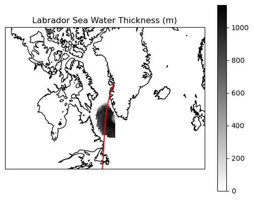
Here is the Labrador Sea Water on a map…
Show code cell source
iy =72
ax = plt.axes(projection=ccrs.LambertConformal(central_longitude=-50.0, central_latitude=55.0))
# for fc in [2,6,10]
plt.pcolormesh(ds.XC[10],ds.YC[10],
               (ds.drF*mode_water[:,10]).sum(dim = 'Z'),
               cmap = "binary",
               transform = ccrs.PlateCarree())
plt.plot(ds.XC[10,iy],ds.YC[10,iy],color = 'r',transform = ccrs.PlateCarree())
ax.set_extent([-100,-10,45,80],crs = ccrs.PlateCarree())
plt.colorbar()
ax.coastlines()
ax.set_title('Labrador Sea Water Thickness (m)')
Text(0.5, 1.0, 'Labrador Sea Water Thickness (m)')
… and at a vertical section:
Show code cell source
iy = 72
section = np.array(ds.S_bar[:,10,iy])
section[section==0] = np.nan
plt.pcolormesh(ds.YC[10,iy],ds.Z,section,vmax = 35,vmin = 34.5)
plt.colorbar()
plt.contour(ds.YC[10,iy],ds.Z,mode_water[:,10,iy])
plt.xlim(52,70)
plt.ylim(-3700,0)
plt.title('Vertical Section along the Red Line')
Text(0.5, 1.0, 'Vertical Section along the Red Line')
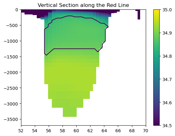
Vertical Section at the red line. The shading shows salinity, and the contours shows the location of Labrador Sea Water
2. Simulate particle trajectories#
Now we create a Particle object. There are a couple of keyword arguments that are worth noticing:
bool_array+numis an alternative way to initialize particle without specifying x,y,z. The code will randomly place aboutnumparticles uniformly wherebool_arrayis True. You can also pass a float array intobool_arrayto give it some weight.random_seedis optional.save_raw=Trueto record every grid cell crossing, this is essential for closing budgettransport = Trueto have the u,v,w variables interpreted as volume flux.
p = sd.Particle(
    bool_array=mode_water, num=3000, random_seed=0,
    t = 5e7,
    data = tub, free_surface = 'noflux',
    save_raw = True,uname = 'utrans',vname = 'vtrans',wname = 'wtrans',
    transport  = True
)
To minimize the runtime and the storage demand, we only put about 3000 particles (not exactly), and each particle represent a fairly large volume.
vol_each = float((ds.drF*ds.rA*ds.hFacC*mode_water[:,10]).sum())/p.N/1e9
print('Each particle represent a volume of:',vol_each, 'km³')
print(f'There is a total of {p.N} particles.')
Each particle represent a volume of: 1660.4962036023273 km³
There is a total of 3066 particles.
You probably noticed that we set t = 5e7 seconds, or about 1.58 years when we initiated Particle. Since the velocity field is time-independent, we only care about the duration rather than the absolute value of time. Let’s simulated the Particle back for 1.58 years to reach t=0.
stops = [0]
Now, we simulate the particles. dump_filename will let the code know to save it in a file.
I highly recommend that you preserve_checks for reasons that will be obvious shortly after, especially when you run it for the first time.
p.to_list_of_time(normal_stops = stops,
                  dump_filename = 'ls_mode_water_',
                  store_kwarg = {'preserve_checks':True})
1970-01-01T00:00:00
3. Budget on trajectories#
first we load the file we stored:
traj = xr.open_zarr('ls_mode_water_1970-01-01T00:00:00')
traj
<xarray.Dataset> Size: 51MB
Dimensions:  (nprof: 320164, five: 5, shapes: 3066)
Coordinates:
  * nprof    (nprof) int64 3MB 0 1 2 3 4 ... 320159 320160 320161 320162 320163
  * five     (five) <U4 80B 'iw' 'iz' 'face' 'iy' 'ix'
  * shapes   (shapes) int64 25kB 172 64 60 54 58 40 50 ... 88 58 56 64 120 178
Data variables: (12/22)
    du       (nprof) float64 3MB dask.array<chunksize=(40021,), meta=np.ndarray>
    dv       (nprof) float64 3MB dask.array<chunksize=(40021,), meta=np.ndarray>
    dw       (nprof) float64 3MB dask.array<chunksize=(40021,), meta=np.ndarray>
    face     (nprof) int16 640kB dask.array<chunksize=(160082,), meta=np.ndarray>
    frac     (nprof) float64 3MB dask.array<chunksize=(40021,), meta=np.ndarray>
    ind1     (five, nprof) int16 3MB dask.array<chunksize=(2, 80041), meta=np.ndarray>
    ...       ...
    vs       (nprof) int16 640kB dask.array<chunksize=(160082,), meta=np.ndarray>
    vv       (nprof) float64 3MB dask.array<chunksize=(40021,), meta=np.ndarray>
    ww       (nprof) float64 3MB dask.array<chunksize=(40021,), meta=np.ndarray>
    xx       (nprof) float64 3MB dask.array<chunksize=(40021,), meta=np.ndarray>
    yy       (nprof) float64 3MB dask.array<chunksize=(40021,), meta=np.ndarray>
zz (nprof) float64 3MB dask.array<chunksize=(40021,), meta=np.ndarray>nprof is an index of all the instances of particle crossing grid cell wall+the beginning and the end of the time step. shapes tell you how many such instances happen for each particles.
Now, a very important step. check if what we have done so far is correct. We calculate \(-\nabla \cdot (US)\) from traj using the extra variables we saved when we preserve_checks and compare that to the Eulerian budget we calculated earlier.
ans,_ = sd.lagrangian_budget.check_particle_data_compat(traj,ds,
                                                        p.tp,
                                                        wall_names=('sx_bar','sy_bar','sz_bar'),
                                                        conv_name = 'conv_us',
                                                        debug = True)
assert ans,'If the assert statement failed, _ contains some debugging info. '
If ans = False, ask yourself the following questions:
Does your Eulerian \(-\nabla \cdot (US)\) close the budget?
Did you use the same volume transport (including bolus velocity) to calculate Eulerian budget and simulate particles?
Is
tub['Vol']in this notebook the same as the one used in the Eulerian budget?(If you are running time-dependent simulations) Does the time step of the particle trajectory match that of the budget? ….
If you answer is yes to all of those questions, and ans is still False. Raise an issue on GitHub.
OK, now I am going to assume you pass the check:
I am so glad to hear that the checks passed! I am very proud of you! Now you can rest assured that we are performing the Lagrangian budget correctly.
All of our effort has brought us to this point. We have the trajectory and the budget. Just pass in the variable names of the RHS terms, the Eulerian tendency term, and the wall salinity, and the budget is calculated!
walls_names = dict(xname="sx_bar", yname="sy_bar", zname="sz_bar")
contr_dic, s, first, last = sd.lagrangian_budget.calculate_budget(traj, ds,
                                                                  rhs_list,
                                                                  prefetch_vector_kwarg = walls_names,
                                                                  lhs_name = 'tend_s')
contr_dic is the main result, a dictionary containing the contribution of each RHS terms.
s is the salinity recorded at each boundary crossing.
first and last are indices of where the record of a single particle begins and ends, as illustrated here

s, all variables in traj and contr_dic are all one dimensional arrays. To retrieve the information of the ith (or i+1 if you count from 1) particle, one simply do contr_dic[var][first[i]:last[i]+1]
4. Visualizing the results#
There are several ways to visualize the budget results.
Show code cell source
maps = {}
for var in rhs_list+['count']:
    maps[var] = np.zeros((50,13,90,90))


def cumu_map_array(traj, value):
    ind = tuple(np.array(i)[:-1] for i in [traj.iz-1, traj.face, traj.iy, traj.ix])
    array = np.zeros((50,13,90,90))
    np.add.at(array, ind, value)
    return array


for var in rhs_list:
    maps[var] += cumu_map_array(traj, contr_dic[var])
    maps['count'] += cumu_map_array(traj, np.ones_like(contr_dic['forc_s']))

maps_ds = xr.Dataset()
for var in rhs_list+['count']:
    maps_ds[var] = xr.DataArray(maps[var],dims = ('Z','face','Y','X'))
Show code cell source
ip = 0
ax = plt.axes(projection=ccrs.LambertConformal(central_longitude=-50.0, central_latitude=55.0))
for fc in [2,6,10]:
    data_face = -maps_ds['count'][:, fc].sum(dim="Z")

    m1 = ax.pcolormesh(
        ds.XC[fc], ds.YC[fc],
        data_face,
        cmap='Blues_r',
        transform=ccrs.PlateCarree(),
        zorder = 0
    )
for ip in range(0,p.N,100):
    plt.plot(traj.xx[first[ip]:last[ip]],traj.yy[first[ip]:last[ip]],
             color = 'gold',alpha = 0.3,
             zorder  =10,transform = ccrs.PlateCarree())

ax.set_extent([-100,-10,45,80],crs = ccrs.PlateCarree())
ax.coastlines()
<cartopy.mpl.feature_artist.FeatureArtist at 0x7f3f59fbd710>
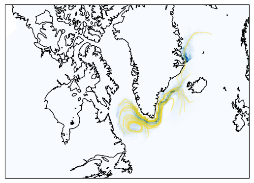
The yellow lines shows a subset of the particle trajectories. The shadings are the count of grid cell crossings.
You can use the indices stored in traj to generate a “map of contribution”.
Show code cell source
cmap = "PuOr_r"
vmax = 1
fig = plt.figure(figsize=(10, 9))
gs = gridspec.GridSpec(
    3, 2,
    height_ratios=[1, 1, 0.08],
    hspace=0.15,
    wspace=0.05
)

axes = []
for i in range(2):
    for j in range(2):
        ax = fig.add_subplot(
            gs[i, j],
            projection=ccrs.LambertConformal(central_longitude=-50.0, central_latitude=55.0)
        )
        axes.append(ax)
mappable = None

for ax, var in zip(axes, rhs_list):
    for fc in [2,6,10]:
        data_face = -maps_ds[var][:, fc].sum(dim="Z")*vol_each*1e6/ds.rA[fc]
        m1 = ax.pcolormesh(
            ds.XC[fc], ds.YC[fc],
            data_face,
            cmap=cmap,
            vmax = vmax,
            vmin = -vmax,
            transform=ccrs.PlateCarree()
        )
    ax.coastlines()
    ax.set_title(longname[var])
    ax.set_extent([-100,-10,45,80],crs = ccrs.PlateCarree())

    if mappable is None:
        mappable = m1

cax = fig.add_subplot(gs[2, :])
cbar = fig.colorbar(
    mappable,
    cax=cax,
    extend = 'both',
    aspect = 40,
    orientation="horizontal"
)
cbar.set_label(r'$PSU\cdot km$')
plt.show()
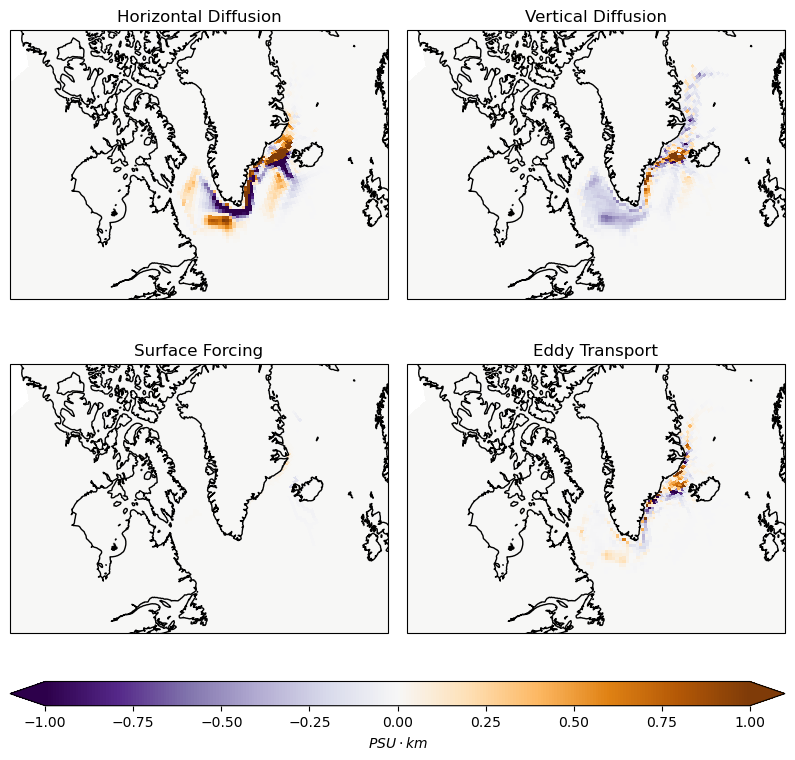
The map of each terms to the overall salinity change. The unit is \(PSU\cdot km\) because we integrate in the vertical. Blue means the water is freshened.
5. Budget closure revisited.#
You can also average over all the particles to see what the contribution of each terms are.
Show code cell source
total = 0
for var in rhs_list:
    change = -sum(contr_dic[var]/p.N)
    print(f'Salinity Change due to {longname[var]}: {change} PSU')
    total+=change
print(f'Sum of all terms: {total}')
Salinity Change due to Horizontal Diffusion: 0.012515693718306607 PSU
Salinity Change due to Vertical Diffusion: -0.02401320107054221 PSU
Salinity Change due to Surface Forcing: 0.00018392443083714758 PSU
Salinity Change due to Eddy Transport: 0.005359598102315094 PSU
Sum of all terms: -0.005953984819083361
The change of salinity can also be calculated by taking the difference between the beginning and the end
Show code cell source
print('The total change of salinity:', (s[first].mean() - s[last].mean()))
The total change of salinity: -0.006020058739906631
There is about a 1% mismatch, and that is because of the linear freshening trend!
Show code cell source
var = 'tend_s'
change = -sum(contr_dic[var]/p.N)
print(f'Salinity Change due to Eulerian Tendency: {change} PSU')
Salinity Change due to Eulerian Tendency: -7.239317959637215e-05 PSU