This dataset contains three variables: sea surface height (ETAN, in meters), velocity in the x-direction (UVELMASS, in meters per second) and velocity in the y-direction (VVELMASS, in meters per second). This slice of data is a single snapshot in time - that is, it contains only one time point.
It is useful to note that ASTE uses complex grid topology, such that it has a face dimension as well as X and Y dimensions.
💡 Note: The full ASTE dataset can be accessed using xmitgcm by following instructions
here.
This notebook will describe how to put some particles in the Arctic Ocean and visualize their movements for six months. To do this, seaduck requires that the ASTE data is in the form of a seaduck Ocean Dataset. This allows for conversion between grid coordinates and latitude/longitude coordinates, as well as providing topology information.
bathtub=sd.OceData(ds)bathtub
<seaduck.ocedata.OceData at 0x7f4088ebf290>
The above code cell generated the seaduck Ocean Dataset object. This object includes a topology object, which for ASTE is of type ‘LLC’. This reflects ASTE’s Latitude-Longitude-Cap grid.
bathtub.tp.typ
'LLC'
Now that the dataset for the interpolation has been prepared, we can initialize particles in the Arctic Ocean. We need to decide where and when the particle trajectories will begin.
For this example, we will place particles randomly all over the Arctic Ocean. This code generates particles distributed on a sphere further north than 70 degrees latitude, all with a depth of 10m.
N=int(10e4)np.random.seed(0)# Reset seed for reproducability# Place particles on a sphere with normal distribution in x, y and zxx,yy,zz=[np.random.normal(size=N)foriinrange(3)]r=np.sqrt(xx**2+yy**2+zz**2)y=(np.pi/2-np.arccos(zz/r))*180/np.pix=np.arctan2(yy,xx)*180/np.pi# Limit to be further north than 70 degrees latitudex=x[y>70]y=y[y>70]# Set depth to be -10 metresz=np.ones_like(x)*(-10.0)
Next, we will consider the timing of the simulation. The ASTE data used here begins on 1st February 2002, so this must be the starting time, t. However, this dataset is a snapshot, and does not have a true time dimension.
We will also need to choose for how long we would like to simulate our particles. Because the dataset has no true time dimension, we must think of time relatively rather than absolutely. Let’s choose to simulate these particles forwards in time for six months, such that the end time is 2002-08-01. This means that the particles will move about for six months using the velocities stored in ds.
t=np.ones_like(x)*sd.utils.convert_time("2002-02-01")# Initial timetf=sd.utils.convert_time("2002-08-01")# Final time
It’s good practice to set a limit at which particles stop being tracked. This can speed up the simulation, and help make output data more manageable. This example will stop tracking particles once they cross the 60 degree parallel.
definterested_in(p):return60<p.lat
Now that all of the set up has been taken care of, we can create a Particle object! This allows us to combine all the initial information about the particles (e.g. spatial distribution, time) in one object that can be used to integrate the particles in time.
p=sd.Particle(x=x,y=y,z=z,t=t,data=bathtub,uname="UVELMASS",vname="VVELMASS",wname=None,callback=interested_in,)# remove particles on land.p=p.subset(p.u!=0)# Inspect the objectp
<seaduck.lagrangian.Particle at 0x7f40e01be450>
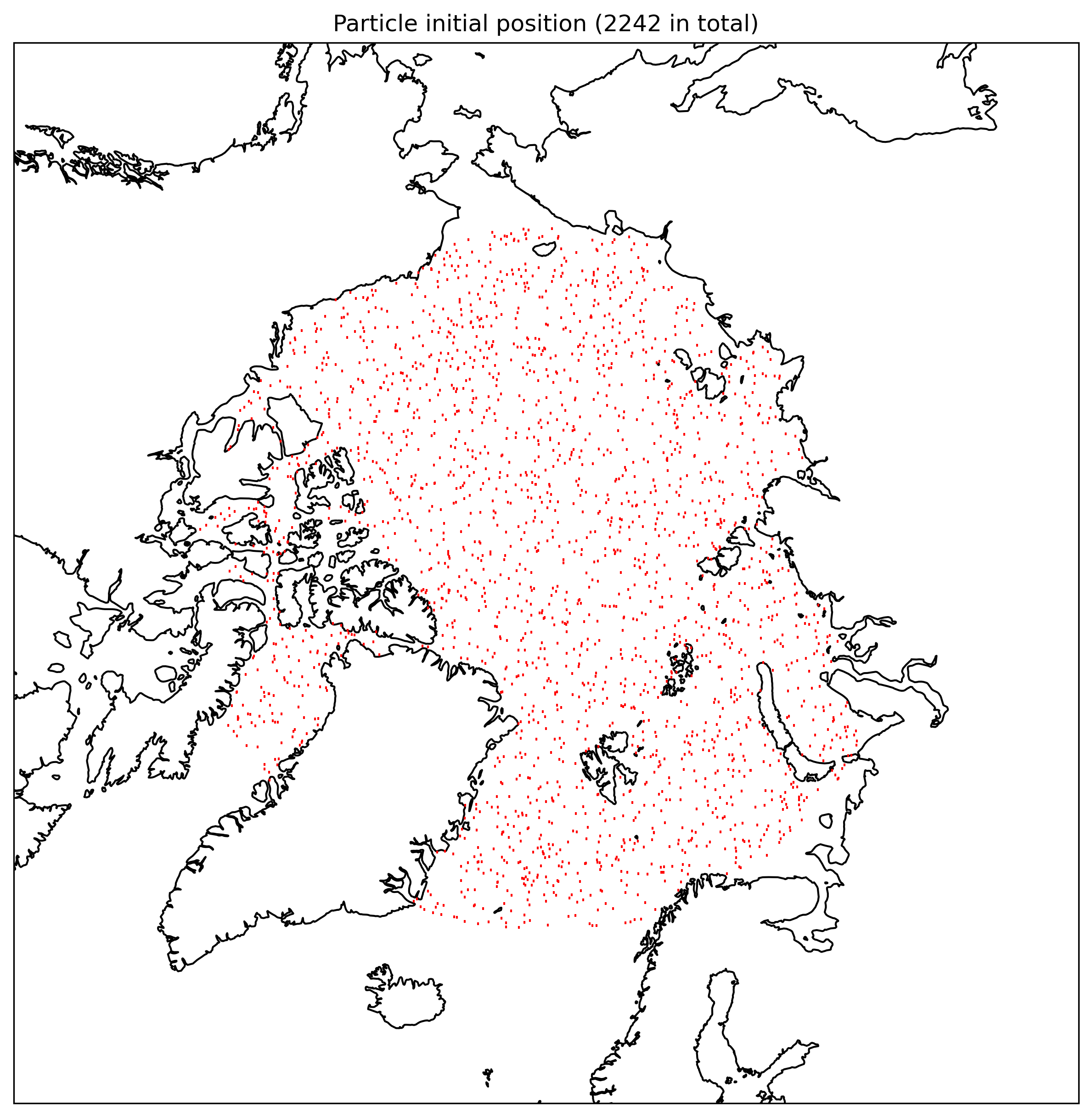
Let’s check out the inital positions of our particles.
plt.figure(figsize=(10,10))ax=plt.axes(projection=ccrs.NorthPolarStereo(central_longitude=0))ax.plot(p.lon,p.lat,"r+",markersize=1,transform=ccrs.PlateCarree())ax.coastlines()ax.set_extent([-180,180,60,90],ccrs.PlateCarree())ax.set_title(f"Particle initial position ({p.N} in total)")plt.show()
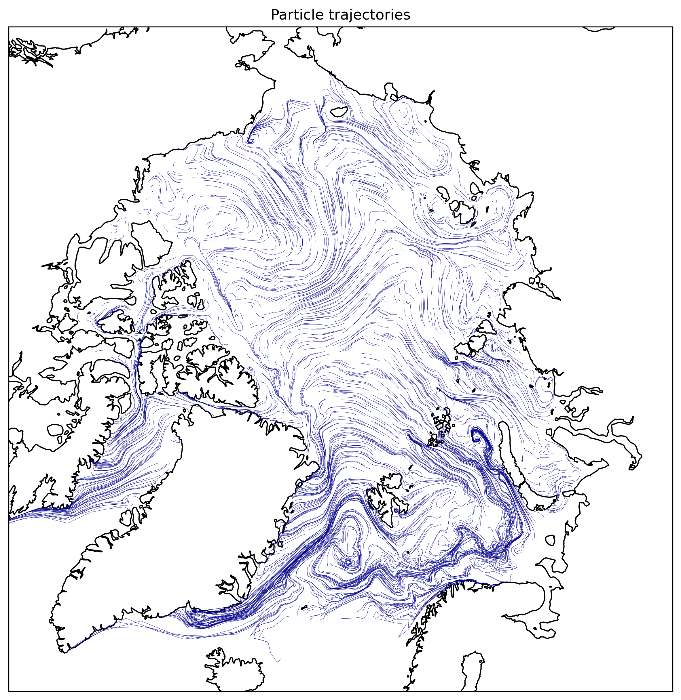
The particles are in position, so it is time to carry out the simulation. Seaduck’s Particle object has the .to_list_of_time option, which runs the particle trajectory simulation and returns the particle positions at specified output times. These output times are defined by normal_stops, at 15 regular intervals between the beginning time, t[0], and the end time, tf. We will generate stops, which is a list of time that corresponds to normal_stops, and raw, which is a list of sd.Position objects, one for each time in stops.
# Define when to dump outputnormal_stops=np.linspace(t[0],tf,15)# Simulation!stops,raw=p.to_list_of_time(normal_stops=normal_stops)