Horizontal stream function conservation

author, Wenrui Jiang 06/06/2022

This package currently only supports velocity fields that are piecewise stationary in time. For a stable velocity field, the streaklines will match the streamlines of the field.

For 2D cases, this means conservation of stream function.

\[ \frac{d \Psi}{dt} = 0 \]

A strong test can be constructed as follows: simulate the particles under an arbitrary stream function and compare the stream function before-and-after. If the code is correct, the stream function defined at the starting position of a particle should match that defined at the final position.

Show code cell source Hide code cell source

import warnings

import matplotlib as mpl
import matplotlib.pyplot as plt
import numpy as np
import pooch
import xarray as xr
from matplotlib import cm, colors

import seaduck as sd

mpl.rcParams["figure.dpi"] = 300

warnings.filterwarnings("ignore")

Loading data

For this test example, the stream function we are going to use is an award-winning eddy in the arbitrary/cute department. Let’s load it.

file_path = pooch.retrieve(
    url="https://github.com/MaceKuailv/seaduck_sciserver_notebook/raw/master/diffused_duck.npy",
    known_hash="8968fc89a57a492879dff6b458ffa1e03bb533e82bd76ca5db8496182fa2c32f",
)

strmf = np.load(file_path)[::-1]
M, N = strmf.shape
M -= 1
N -= 1
x = np.linspace(-1, 1, N + 1)
y = np.linspace(-1, 1, M + 1)
xg, yg = np.meshgrid(x, y)

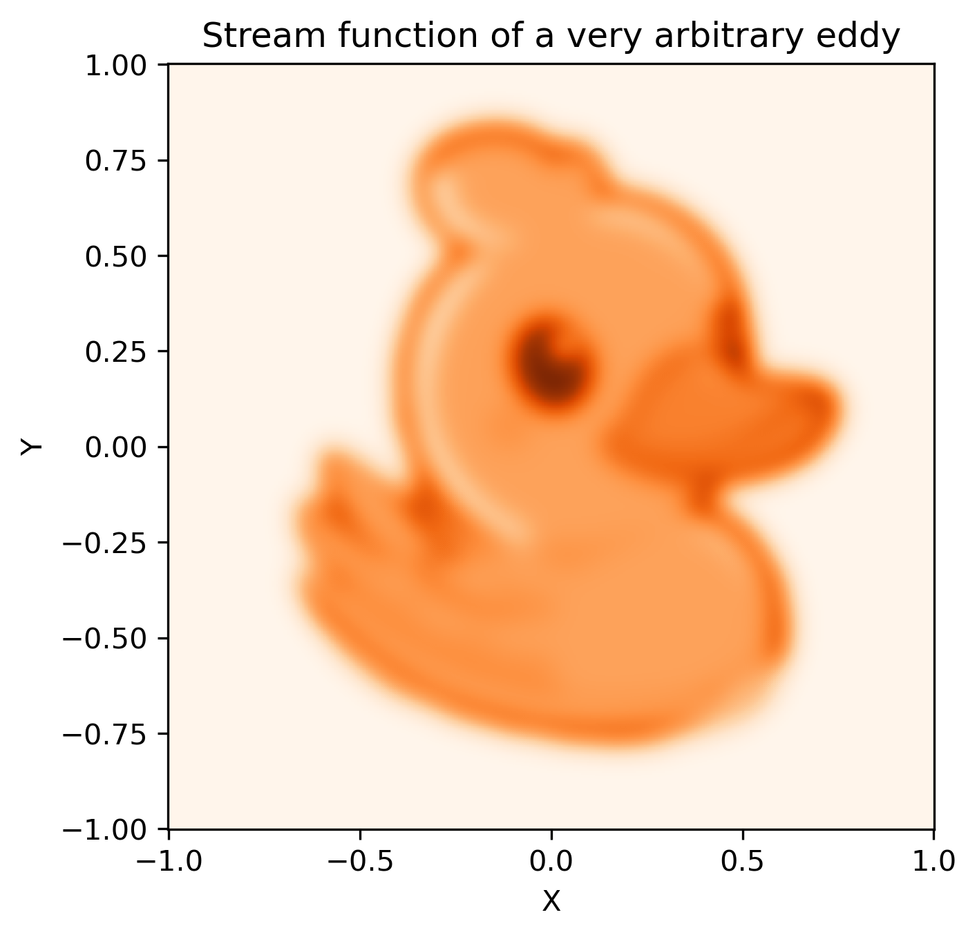
To show that I am not volkswagening you, I will plot the stream function.

plt.pcolormesh(xg, yg, strmf, cmap="Oranges")
plt.gca().set_aspect("equal")
plt.xlabel("X")
plt.ylabel("Y")
plt.title("Stream function of a very arbitrary eddy")
plt.show()

Fig.1 A stream function that is not particular in any senses.

Now we prepare create the grids needed and therefore the xarray dataset for the simulation.

Show code cell source Hide code cell source

xv = 0.5 * (xg[:, 1:] + xg[:, :-1])
yv = 0.5 * (yg[:, 1:] + yg[:, :-1])
xu = 0.5 * (xg[1:] + xg[:-1])
yu = 0.5 * (yg[1:] + yg[:-1])

xc = 0.5 * (xv[1:] + xv[:-1])
yc = 0.5 * (yv[1:] + yv[:-1])

u = np.diff(strmf, axis=0)
v = -np.diff(strmf, axis=1)

Show code cell source Hide code cell source

ds = xr.Dataset(
    coords=dict(
        XC=(["Y", "X"], xc),
        YC=(["Y", "X"], yc),
        XG=(["Yp1", "Xp1"], xg),
        YG=(["Yp1", "Xp1"], yg),
        rA=(["Y", "X"], np.ones_like(xc, float)),
    ),
    data_vars=dict(
        UVELMASS=(["Y", "Xp1"], u),
        VVELMASS=(["Yp1", "X"], v),
        streamfunc=(["Yp1", "Xp1"], strmf),
    ),
)
ds

<xarray.Dataset> Size: 31MB
Dimensions:     (Y: 699, Xp1: 700, Yp1: 700, X: 699)
Coordinates:
    XC          (Y, X) float64 4MB -0.9986 -0.9957 -0.9928 ... 0.9957 0.9986
    YC          (Y, X) float64 4MB -0.9986 -0.9986 -0.9986 ... 0.9986 0.9986
    XG          (Yp1, Xp1) float64 4MB -1.0 -0.9971 -0.9943 ... 0.9971 1.0
    YG          (Yp1, Xp1) float64 4MB -1.0 -1.0 -1.0 -1.0 ... 1.0 1.0 1.0 1.0
    rA          (Y, X) float64 4MB 1.0 1.0 1.0 1.0 1.0 ... 1.0 1.0 1.0 1.0 1.0
Dimensions without coordinates: Y, Xp1, Yp1, X
Data variables:
    UVELMASS    (Y, Xp1) float64 4MB 0.0 0.0 0.0 ... -1.616e-78 -2.363e-83 0.0
    VVELMASS    (Yp1, X) float64 4MB -0.0 -0.0 -0.0 -0.0 ... -0.0 -0.0 -0.0 -0.0
    streamfunc  (Yp1, Xp1) float64 4MB 0.0 0.0 0.0 0.0 0.0 ... 0.0 0.0 0.0 0.0

xarray.Dataset

• Dimensions:
  • Y: 699
  • Xp1: 700
  • Yp1: 700
  • X: 699
• Coordinates: (5)
  • XC
    (Y, X)
    float64
    -0.9986 -0.9957 ... 0.9957 0.9986

    array([[-0.99856938, -0.99570815, -0.99284692, ...,  0.99284692,
             0.99570815,  0.99856938],
           [-0.99856938, -0.99570815, -0.99284692, ...,  0.99284692,
             0.99570815,  0.99856938],
           [-0.99856938, -0.99570815, -0.99284692, ...,  0.99284692,
             0.99570815,  0.99856938],
           ...,
           [-0.99856938, -0.99570815, -0.99284692, ...,  0.99284692,
             0.99570815,  0.99856938],
           [-0.99856938, -0.99570815, -0.99284692, ...,  0.99284692,
             0.99570815,  0.99856938],
           [-0.99856938, -0.99570815, -0.99284692, ...,  0.99284692,
             0.99570815,  0.99856938]])

  • YC
    (Y, X)
    float64
    -0.9986 -0.9986 ... 0.9986 0.9986

    array([[-0.99856938, -0.99856938, -0.99856938, ..., -0.99856938,
            -0.99856938, -0.99856938],
           [-0.99570815, -0.99570815, -0.99570815, ..., -0.99570815,
            -0.99570815, -0.99570815],
           [-0.99284692, -0.99284692, -0.99284692, ..., -0.99284692,
            -0.99284692, -0.99284692],
           ...,
           [ 0.99284692,  0.99284692,  0.99284692, ...,  0.99284692,
             0.99284692,  0.99284692],
           [ 0.99570815,  0.99570815,  0.99570815, ...,  0.99570815,
             0.99570815,  0.99570815],
           [ 0.99856938,  0.99856938,  0.99856938, ...,  0.99856938,
             0.99856938,  0.99856938]])

  • XG
    (Yp1, Xp1)
    float64
    -1.0 -0.9971 -0.9943 ... 0.9971 1.0

    array([[-1.        , -0.99713877, -0.99427754, ...,  0.99427754,
             0.99713877,  1.        ],
           [-1.        , -0.99713877, -0.99427754, ...,  0.99427754,
             0.99713877,  1.        ],
           [-1.        , -0.99713877, -0.99427754, ...,  0.99427754,
             0.99713877,  1.        ],
           ...,
           [-1.        , -0.99713877, -0.99427754, ...,  0.99427754,
             0.99713877,  1.        ],
           [-1.        , -0.99713877, -0.99427754, ...,  0.99427754,
             0.99713877,  1.        ],
           [-1.        , -0.99713877, -0.99427754, ...,  0.99427754,
             0.99713877,  1.        ]])

  • YG
    (Yp1, Xp1)
    float64
    -1.0 -1.0 -1.0 -1.0 ... 1.0 1.0 1.0

    array([[-1.        , -1.        , -1.        , ..., -1.        ,
            -1.        , -1.        ],
           [-0.99713877, -0.99713877, -0.99713877, ..., -0.99713877,
            -0.99713877, -0.99713877],
           [-0.99427754, -0.99427754, -0.99427754, ..., -0.99427754,
            -0.99427754, -0.99427754],
           ...,
           [ 0.99427754,  0.99427754,  0.99427754, ...,  0.99427754,
             0.99427754,  0.99427754],
           [ 0.99713877,  0.99713877,  0.99713877, ...,  0.99713877,
             0.99713877,  0.99713877],
           [ 1.        ,  1.        ,  1.        , ...,  1.        ,
             1.        ,  1.        ]])

  • rA
    (Y, X)
    float64
    1.0 1.0 1.0 1.0 ... 1.0 1.0 1.0 1.0

    array([[1., 1., 1., ..., 1., 1., 1.],
           [1., 1., 1., ..., 1., 1., 1.],
           [1., 1., 1., ..., 1., 1., 1.],
           ...,
           [1., 1., 1., ..., 1., 1., 1.],
           [1., 1., 1., ..., 1., 1., 1.],
           [1., 1., 1., ..., 1., 1., 1.]])

• Data variables: (3)
  • UVELMASS
    (Y, Xp1)
    float64
    0.0 0.0 0.0 ... -2.363e-83 0.0

    array([[ 0.00000000e+00,  0.00000000e+00,  0.00000000e+00, ...,
             5.62852688e-66,  5.57579561e-67,  0.00000000e+00],
           [ 0.00000000e+00,  0.00000000e+00,  0.00000000e+00, ...,
             4.87304737e-66,  3.95612555e-66,  0.00000000e+00],
           [ 0.00000000e+00,  0.00000000e+00,  0.00000000e+00, ...,
             6.49687727e-65,  3.41435180e-66,  0.00000000e+00],
           ...,
           [ 0.00000000e+00,  0.00000000e+00,  0.00000000e+00, ...,
            -3.57996441e-77,  1.20108218e-78,  0.00000000e+00],
           [ 0.00000000e+00,  0.00000000e+00,  0.00000000e+00, ...,
             1.61457662e-78, -1.20179182e-78,  0.00000000e+00],
           [ 0.00000000e+00,  0.00000000e+00,  0.00000000e+00, ...,
            -1.61561141e-78, -2.36258439e-83,  0.00000000e+00]])

  • VVELMASS
    (Yp1, X)
    float64
    -0.0 -0.0 -0.0 ... -0.0 -0.0 -0.0

    array([[-0.00000000e+00, -0.00000000e+00, -0.00000000e+00, ...,
            -0.00000000e+00, -0.00000000e+00, -0.00000000e+00],
           [-0.00000000e+00, -0.00000000e+00, -0.00000000e+00, ...,
             6.68997918e-66,  5.07094732e-66,  5.57579561e-67],
           [-0.00000000e+00, -0.00000000e+00, -0.00000000e+00, ...,
             8.59075270e-65,  5.98786914e-66,  4.51370511e-66],
           ...,
           [-0.00000000e+00, -0.00000000e+00, -0.00000000e+00, ...,
             4.89845917e-77, -1.20078067e-78,  1.20181545e-78],
           [-0.00000000e+00, -0.00000000e+00, -0.00000000e+00, ...,
            -1.61423773e-78,  1.61558778e-78,  2.36258439e-83],
           [-0.00000000e+00, -0.00000000e+00, -0.00000000e+00, ...,
            -0.00000000e+00, -0.00000000e+00, -0.00000000e+00]])

  • streamfunc
    (Yp1, Xp1)
    float64
    0.0 0.0 0.0 0.0 ... 0.0 0.0 0.0 0.0

    array([[0.00000000e+00, 0.00000000e+00, 0.00000000e+00, ...,
            0.00000000e+00, 0.00000000e+00, 0.00000000e+00],
           [0.00000000e+00, 0.00000000e+00, 0.00000000e+00, ...,
            5.62852688e-66, 5.57579561e-67, 0.00000000e+00],
           [0.00000000e+00, 0.00000000e+00, 0.00000000e+00, ...,
            1.05015742e-65, 4.51370511e-66, 0.00000000e+00],
           ...,
           [0.00000000e+00, 0.00000000e+00, 0.00000000e+00, ...,
            1.03478322e-81, 1.20181545e-78, 0.00000000e+00],
           [0.00000000e+00, 0.00000000e+00, 0.00000000e+00, ...,
            1.61561141e-78, 2.36258439e-83, 0.00000000e+00],
           [0.00000000e+00, 0.00000000e+00, 0.00000000e+00, ...,
            0.00000000e+00, 0.00000000e+00, 0.00000000e+00]])

• Indexes: (0)
• Attributes: (0)

Prepare for the test

First, we create the seaduck.OceData object

tub = sd.OceData(ds)

Then, initialize the particle position.

num_particle = 8000
np.random.seed(99)
x = np.random.random(num_particle) * 1.6 - 0.8
y = np.random.random(num_particle) * 1.8 - 0.9

pt = sd.Particle(
    x=x, y=y, z=None, t=np.zeros_like(x), data=tub, wname=None, transport=True
)

Finally, we need a proper kernel for interpolating stream function. The natural definition for this case is to interpolate using the four closest corner points.

kkk = np.array([[0, 0], [0, 1], [1, 0], [1, 1]])

gknw = sd.KnW(kkk, vkernel="nearest", tkernel="nearest")

The actual test

First we interpolate the streamfunction at the starting position.

before = pt.interpolate("streamfunc", gknw)

Now, simulate the particles forward for a decent amount of time.

steps = 15
stops, ps = pt.to_list_of_time(
    normal_stops=np.linspace(0, 2 * steps * N, steps), update_stops=[]
)

1970-01-01T00:00:00
1970-01-01T00:24:58
1970-01-01T00:49:56

1970-01-01T01:14:54
1970-01-01T01:39:51

1970-01-01T02:04:49
1970-01-01T02:29:47

1970-01-01T02:54:45
1970-01-01T03:19:43

1970-01-01T03:44:41
1970-01-01T04:09:39

1970-01-01T04:34:36
1970-01-01T04:59:34

1970-01-01T05:24:32
1970-01-01T05:49:30

Now that, the particles are at a different position. Let’s look at the stream functions again and compare.

after = ps[-1].interpolate("streamfunc", gknw)

Show code cell source Hide code cell source

is_it_close = np.allclose(after, before, atol=1e-7)
max_difference = np.max(np.abs(after - before))
print(f"Is the stream function conserved? {is_it_close}")
print(f"The maximum difference is {max_difference }")

Is the stream function conserved? True
The maximum difference is 2.4288904221236862e-12

To put that in perspective: The stream function ranges from 0 to around 0.6. So this is a small difference!

If you’re not convinced

“Hey, you just used your own function to test another function. I didn’t see anything under the hood. “ “Also, the stream function should be conserved along the entire trajectory. Not only the start and the end”

Well, here is a more visual way of proving my points.

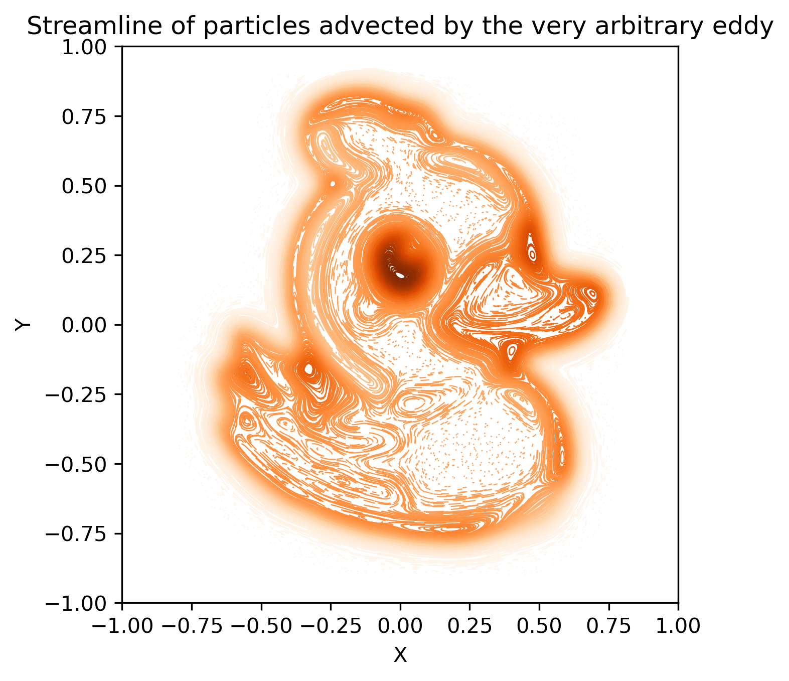
I am going to plot the trajectory of all the particles, and color them using the initial stream function.

If the stream function is not conserved at any point, the color of the lines drawn (initial value of stream function) will not match that we plotted earlier (the actual value defined at that point).

Show code cell source Hide code cell source

lons = []
lats = []
for ppp in ps:
    lons.append(ppp.lon)
    lats.append(ppp.lat)
lons = np.array(lons)
lats = np.array(lats)

Using the same color scheme as the previous plot

norm = colors.Normalize(vmin=0.0, vmax=0.6, clip=True)
mapper = cm.ScalarMappable(norm=norm, cmap=cm.Oranges)

Show code cell source Hide code cell source

for i in range(len(x)):
    plt.plot(lons.T[i], lats.T[i], c=mapper.to_rgba(before[i]), lw=0.55)
plt.gca().set_aspect("equal")
plt.xlim([-1, 1])
plt.ylim([-1, 1])
plt.xlabel("X")
plt.ylabel("Y")
plt.title("Streamline of particles advected by the very arbitrary eddy")
plt.show()

Fig.1 The trajectories of particles advected by the very arbitrary eddy. The color denotes the initial value of stream function.