Tilted solid-body rotation#
If you’ve already looked at the stream function conservation examples in the horizontal and vertical examples, you may still have the following doubts:
What if the flow is not 2D/not aligned with the grid direction?
If the velocity components are all scaled by a factor, the streamlines will still be the same.
This notebook is designed to address those doubts. We use a tilted solid body rotation with known orbit frequency for demonstration. As far as the package is concerned, tilted 2D flow is not different from fully 3D flow.
Show code cell source
import warnings

import matplotlib as mpl
import matplotlib.pyplot as plt
import numpy as np
import pooch
import xarray as xr
from PIL import Image

import seaduck as sd

mpl.rcParams["figure.dpi"] = 300

warnings.filterwarnings("ignore")
Loading data#
First, we prepare the grid of the dataset
Show code cell source
M = 100
N = 100

x = np.linspace(-1, 1, N + 1)
y = np.linspace(-1, 1, M + 1)
dy = y[1] - y[0]
xg, yg = np.meshgrid(x, y)

xv = 0.5 * (xg[:, 1:] + xg[:, :-1])
yv = 0.5 * (yg[:, 1:] + yg[:, :-1])
xu = 0.5 * (xg[1:] + xg[:-1])
yu = 0.5 * (yg[1:] + yg[:-1])

xc = 0.5 * (xv[1:] + xv[:-1])
yc = 0.5 * (yv[1:] + yv[:-1])

zp1 = np.linspace(0, -4, M + 1)
z = 0.5 * (zp1[1:] + zp1[:-1])
zl = zp1[:-1]
drf = np.abs(np.diff(zp1))
Calculate the solid-body velocity in the horizontal directions:
def solid_body(x, y):
    omega = 1
    r = np.hypot(x, y)
    speed = np.zeros_like(x)
    speed = omega * r

    u = -y / r * speed
    v = x / r * speed
    return u, v
u, _ = solid_body(xu, yu)
_, v = solid_body(xv, yv)
We define the angle of the tilt of the velocity field:
angle = np.pi / 6
tan = np.tan(angle)
The vertical velocity is proportional to the \(v\) velocity by the tangent of the angle we just defined:
vc = 0.5 * (v[1:] + v[:-1])
zygrid = drf[0] / dy
w = tan * vc / zygrid
u = np.tile(u, (len(z), 1, 1))
v = np.tile(v, (len(z), 1, 1))
w = np.tile(w, (len(z), 1, 1))
Now, we can assemble the parts to create the xarray.Dataset:
Show code cell source
ds = xr.Dataset(
    coords=dict(
        XC=(["Y", "X"], xc),
        YC=(["Y", "X"], yc),
        XG=(["Yp1", "Xp1"], xg),
        YG=(["Yp1", "Xp1"], yg),
        rA=(["Y", "X"], np.ones_like(xc, float)),
        Zp1=(["Zp1"], zp1),
        Zl=(["Zl"], zl),
        Z=(["Z"], z),
        drF=(["Z"], drf),
    ),
    data_vars=dict(
        UVELMASS=(["Z", "Y", "Xp1"], u),
        VVELMASS=(["Z", "Yp1", "X"], v),
        WVELMASS=(["Zl", "Y", "X"], w),
    ),
)
ds
<xarray.Dataset> Size: 25MB
Dimensions:   (Z: 100, Y: 100, Xp1: 101, Yp1: 101, X: 100, Zl: 100, Zp1: 101)
Coordinates:
  * Z         (Z) float64 800B -0.02 -0.06 -0.1 -0.14 ... -3.86 -3.9 -3.94 -3.98
    drF       (Z) float64 800B 0.04 0.04 0.04 0.04 0.04 ... 0.04 0.04 0.04 0.04
    XG        (Yp1, Xp1) float64 82kB -1.0 -0.98 -0.96 -0.94 ... 0.96 0.98 1.0
    YG        (Yp1, Xp1) float64 82kB -1.0 -1.0 -1.0 -1.0 ... 1.0 1.0 1.0 1.0
    XC        (Y, X) float64 80kB -0.99 -0.97 -0.95 -0.93 ... 0.95 0.97 0.99
    YC        (Y, X) float64 80kB -0.99 -0.99 -0.99 -0.99 ... 0.99 0.99 0.99
    rA        (Y, X) float64 80kB 1.0 1.0 1.0 1.0 1.0 ... 1.0 1.0 1.0 1.0 1.0
  * Zl        (Zl) float64 800B 0.0 -0.04 -0.08 -0.12 ... -3.88 -3.92 -3.96
  * Zp1       (Zp1) float64 808B 0.0 -0.04 -0.08 -0.12 ... -3.92 -3.96 -4.0
Dimensions without coordinates: Y, Xp1, Yp1, X
Data variables:
    UVELMASS  (Z, Y, Xp1) float64 8MB 0.99 0.99 0.99 0.99 ... -0.99 -0.99 -0.99
    VVELMASS  (Z, Yp1, X) float64 8MB -0.99 -0.97 -0.95 -0.93 ... 0.95 0.97 0.99
WVELMASS (Zl, Y, X) float64 8MB -0.2858 -0.28 -0.2742 ... 0.28 0.2858Prepare the test#
As always, convert xarray.Dataset to seaduck.OceData:
tub = sd.OceData(ds)
Now we define the initial position. For reasons that will be clear in a minute, we define the particle on a plane that is parallel to the velocity field.
Show code cell source
n = 64
m = 64
edge = 0.3
x = np.linspace(-edge, edge, n)
y = np.linspace(-edge, edge, m)
x, y = np.meshgrid(x, y)
x = x.ravel()
y = y.ravel()

z = -2 + tan * y
A coloring scheme is defined here to help human eyes to identify the patterns. We also define a function here that allows us to look at the particles along the \(x\), \(y\), and \(z\) axes.
Show code cell source
file_path = pooch.retrieve(
    url="https://github.com/MaceKuailv/seaduck/blob/main/docs/logo.png?raw=true",
    known_hash="bed53271c0356006eb02751040b7a10536b853872de1c728106ee56227b7c0f8",
)
image = Image.open(file_path)
rgb = np.asarray(image)

bins = 1024 // n
particle_color = rgb[::-bins, ::bins].reshape(len(x), 3) / 255


def plot_particle3d(pt, c=particle_color, s=8):
    fig = plt.figure(figsize=(15, 5))
    ax1 = plt.subplot(1, 3, 1)
    ax1.scatter(pt.lat, pt.dep, c=c, s=s)
    ax1.set_ylabel("z")
    ax1.set_xlabel("y")
    ax1.set_title("Y-Z plane")

    ax2 = plt.subplot(1, 3, 2)
    ax2.scatter(pt.lon, pt.dep, c=c, s=s)
    ax2.set_ylabel("z")
    ax2.set_xlabel("x")
    ax2.set_title("X-Z plane")

    ax3 = plt.subplot(1, 3, 3)
    ax3.scatter(pt.lon, pt.lat, c=c, s=s)
    ax3.set_ylabel("y")
    ax3.set_xlabel("x")
    ax3.set_title("X-Y plane")

    return fig
Run the test#
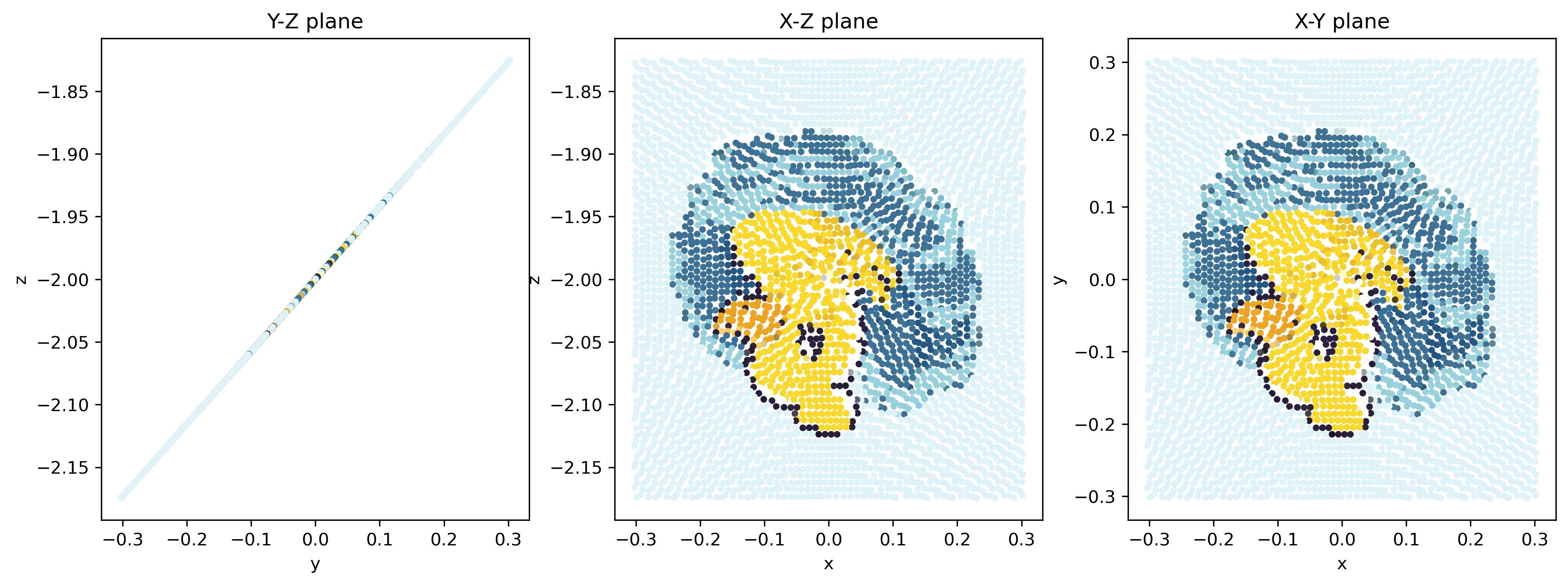
Let’s take a look at the initial condition:
pt = sd.Particle(x=x, y=y, z=z, t=np.zeros_like(x), data=tub, transport=True)
plot_particle3d(pt)
plt.show()

Note that on the \(y\)-\(z\) plane, the particles are aligned on a single straight line.
Now see what happens when we try to run the particles to turn them exactly 180 \(^{\circ}\).
pt.to_next_stop(np.pi * 2)
plot_particle3d(pt)
plt.show()
It turns exactly 180 \(^{\circ}\)! And from the \(y\)-\(z\) plane, it stays a straight line!
You may noticed that the relative position of particles has changed a little. This is because the motion defined by the finite resolution gridded dataset is not a perfect solid-body rotation. However, it is pretty close!
Can you turn it backward a little to get a golden ratio?
pt.to_next_stop(np.pi * 1.618)
plot_particle3d(pt)
plt.show()
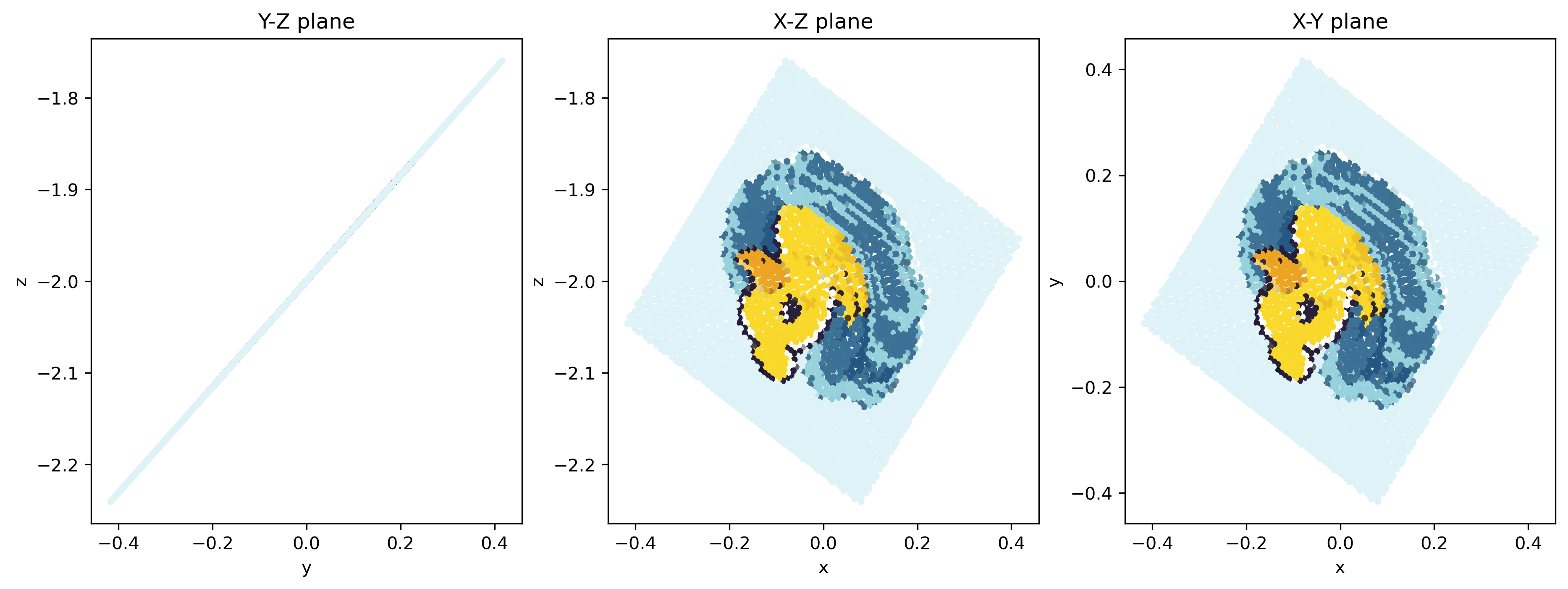
Yes!
What is more impressive is that we can run it back to the initial time. Look what happens:
pt.to_next_stop(0.0)
plot_particle3d(pt)
plt.show()
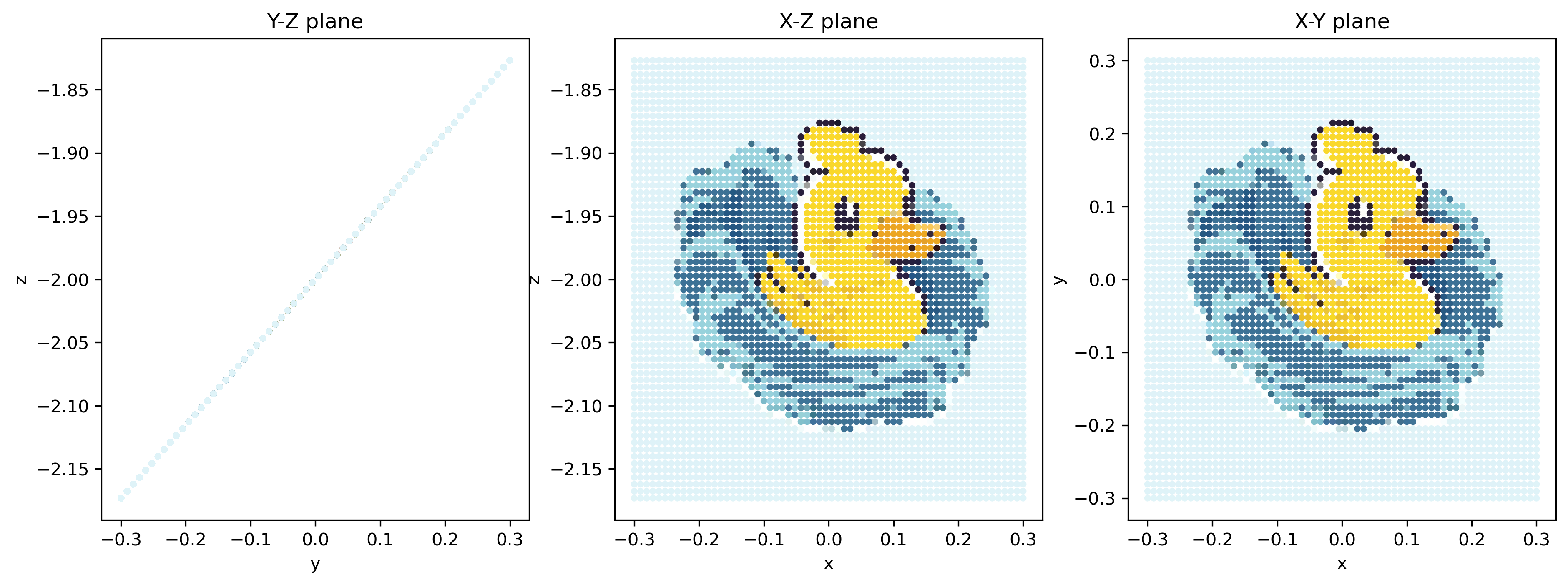
It looks identical to the initial condition!
You have to take my words for it: we did not cache the positions (no cheating!).
Some small errors are introduced during our handling of the particles, so it’s not completely reversible. Let’s check:
np.std(pt.lon - x), np.std(pt.lat - y), np.std(pt.dep - z)
(np.float64(3.2837760975541526e-08),
 np.float64(3.276458147604584e-08),
 np.float64(1.8906243580904905e-08))
But these are pretty small errors!