Topology tutorial

In the movie “Kill Bill”, all the brutal action happens after the main character wakes up from a coma and manages to “wiggle your big toe”. In a similar way, all the functionality of seaduck depends on the Topology class.

As the name “topology” suggests, this object describes how the grids are connected in the horizontal dimensions. This is a simple compact model with high performance. It is also designed with expandability in mind.

For any grid configuration not yet supported by this package, only one function must be added to the code, and, with no (or at least, very little) extra effort, this module (and therefore the entire package) should work for the new configuration.

The magic function is simply: Given a center grid point and its index, if you one want to step one grid point to the up/down/left/right what would the new index be?

And that’s it.

Show code cell source Hide code cell source

import cartopy.crs as ccrs
import matplotlib.pyplot as plt
import numpy as np

import seaduck as sd

For this example, we are going to use ECCO dataset (see also this ECCO notebook). Crucially, this dataset has 13 faces.

ds = sd.utils.get_dataset("ecco")[["UVELMASS", "VVELMASS"]].isel(time=0, Z=0)
ds

<xarray.Dataset> Size: 10MB
Dimensions:   (face: 13, Y: 90, Xp1: 90, Yp1: 90, X: 90)
Coordinates: (12/32)
    CS        (face, Y, X) float32 421kB dask.array<chunksize=(13, 90, 90), meta=np.ndarray>
    Depth     (face, Y, X) float32 421kB dask.array<chunksize=(13, 90, 90), meta=np.ndarray>
    HFacC     (face, Y, X) float32 421kB dask.array<chunksize=(13, 90, 90), meta=np.ndarray>
    HFacS     (face, Yp1, X) float32 421kB dask.array<chunksize=(13, 90, 90), meta=np.ndarray>
    HFacW     (face, Y, Xp1) float32 421kB dask.array<chunksize=(13, 90, 90), meta=np.ndarray>
    PHrefC    float32 4B dask.array<chunksize=(), meta=np.ndarray>
    ...        ...
    rA        (face, Y, X) float32 421kB dask.array<chunksize=(13, 90, 90), meta=np.ndarray>
    rAs       (face, Yp1, X) float32 421kB dask.array<chunksize=(13, 90, 90), meta=np.ndarray>
    rAw       (face, Y, Xp1) float32 421kB dask.array<chunksize=(13, 90, 90), meta=np.ndarray>
    rAz       (face, Yp1, Xp1) float32 421kB dask.array<chunksize=(13, 90, 90), meta=np.ndarray>
    time      datetime64[ns] 8B 1992-01-16T12:00:00
    timestep  int64 8B dask.array<chunksize=(), meta=np.ndarray>
Data variables:
    UVELMASS  (face, Y, Xp1) float64 842kB 0.0 0.0 0.0 0.0 ... 0.0 0.0 0.0 0.0
    VVELMASS  (face, Yp1, X) float64 842kB 0.0 0.0 0.0 0.0 ... 0.0 0.0 0.0 0.0
Attributes: (12/16)
    OceanSpy_description:       ECCO v4r4 3D dataset, ocean simulations on LL...
    OceanSpy_face_connections:  {'face': {0: {'X': ((12, 'Y', False), (3, 'X'...
    OceanSpy_grid_coords:       {'Y': {'Y': None, 'Yp1': -0.5}, 'X': {'X': No...
    OceanSpy_name:              ECCO_v4r4
    OceanSpy_parameters:        {'rSphere': 6371.0, 'eq_state': 'jmd95', 'rho...
    date_created:               Mon Dec 30 11:13:26 2019
    ...                         ...
    geospatial_vertical_max:    -5.0
    geospatial_vertical_min:    -5906.25
    nx:                         90
    ny:                         90
    nz:                         50
    title:                      ECCOv4 MITgcm grid information

xarray.Dataset

• Dimensions:
  • face: 13
  • Y: 90
  • Xp1: 90
  • Yp1: 90
  • X: 90
• Coordinates: (32)
  • CS
    (face, Y, X)
    float32
    dask.array<chunksize=(13, 90, 90), meta=np.ndarray>

    coordinate :

    YC XC

    long_name :

    AngleCS

    units :

    Array Chunk Bytes 411.33 kiB 411.33 kiB Shape (13, 90, 90) (13, 90, 90) Dask graph 1 chunks in 2 graph layers Data type float32 numpy.ndarray

  • Depth
    (face, Y, X)
    float32
    dask.array<chunksize=(13, 90, 90), meta=np.ndarray>

    coordinate :

    XC YC

    long_name :

    ocean depth

    standard_name :

    ocean_depth

    units :

    m

    Array Chunk Bytes 411.33 kiB 411.33 kiB Shape (13, 90, 90) (13, 90, 90) Dask graph 1 chunks in 2 graph layers Data type float32 numpy.ndarray

  • HFacC
    (face, Y, X)
    float32
    dask.array<chunksize=(13, 90, 90), meta=np.ndarray>

    long_name :

    vertical fraction of open cell

    standard_name :

    cell_vertical_fraction

    units :

    Array Chunk Bytes 411.33 kiB 411.33 kiB Shape (13, 90, 90) (13, 90, 90) Dask graph 1 chunks in 3 graph layers Data type float32 numpy.ndarray

  • HFacS
    (face, Yp1, X)
    float32
    dask.array<chunksize=(13, 90, 90), meta=np.ndarray>

    long_name :

    vertical fraction of open cell

    standard_name :

    cell_vertical_fraction_at_v_location

    units :

    Array Chunk Bytes 411.33 kiB 411.33 kiB Shape (13, 90, 90) (13, 90, 90) Dask graph 1 chunks in 3 graph layers Data type float32 numpy.ndarray

  • HFacW
    (face, Y, Xp1)
    float32
    dask.array<chunksize=(13, 90, 90), meta=np.ndarray>

    long_name :

    vertical fraction of open cell

    standard_name :

    cell_vertical_fraction_at_u_location

    units :

    Array Chunk Bytes 411.33 kiB 411.33 kiB Shape (13, 90, 90) (13, 90, 90) Dask graph 1 chunks in 3 graph layers Data type float32 numpy.ndarray

  • PHrefC
    ()
    float32
    dask.array<chunksize=(), meta=np.ndarray>

    long_name :

    Reference Hydrostatic Pressure

    standard_name :

    cell_reference_pressure

    units :

    m2 s-2

    Array Chunk Bytes 4 B 4 B Shape () () Dask graph 1 chunks in 3 graph layers Data type float32 numpy.ndarray

  • SN
    (face, Y, X)
    float32
    dask.array<chunksize=(13, 90, 90), meta=np.ndarray>

    coordinate :

    YC XC

    long_name :

    AngleSN

    units :

    Array Chunk Bytes 411.33 kiB 411.33 kiB Shape (13, 90, 90) (13, 90, 90) Dask graph 1 chunks in 2 graph layers Data type float32 numpy.ndarray

  • X
    (X)
    int64
    0 1 2 3 4 5 6 ... 84 85 86 87 88 89

    axis :

    X

    long_name :

    x-dimension of the t grid

    swap_dim :

    XC

    array([ 0,  1,  2,  3,  4,  5,  6,  7,  8,  9, 10, 11, 12, 13, 14, 15, 16, 17,
           18, 19, 20, 21, 22, 23, 24, 25, 26, 27, 28, 29, 30, 31, 32, 33, 34, 35,
           36, 37, 38, 39, 40, 41, 42, 43, 44, 45, 46, 47, 48, 49, 50, 51, 52, 53,
           54, 55, 56, 57, 58, 59, 60, 61, 62, 63, 64, 65, 66, 67, 68, 69, 70, 71,
           72, 73, 74, 75, 76, 77, 78, 79, 80, 81, 82, 83, 84, 85, 86, 87, 88, 89])

  • XC
    (face, Y, X)
    float32
    dask.array<chunksize=(13, 90, 90), meta=np.ndarray>

    coordinate :

    YC XC

    long_name :

    longitude

    units :

    degrees_east

    Array Chunk Bytes 411.33 kiB 411.33 kiB Shape (13, 90, 90) (13, 90, 90) Dask graph 1 chunks in 2 graph layers Data type float32 numpy.ndarray

  • XG
    (face, Yp1, Xp1)
    float32
    dask.array<chunksize=(13, 90, 90), meta=np.ndarray>

    coordinate :

    YG XG

    long_name :

    longitude

    units :

    degrees_east

    Array Chunk Bytes 411.33 kiB 411.33 kiB Shape (13, 90, 90) (13, 90, 90) Dask graph 1 chunks in 2 graph layers Data type float32 numpy.ndarray

  • Xp1
    (Xp1)
    int64
    0 1 2 3 4 5 6 ... 84 85 86 87 88 89

    axis :

    X

    c_grid_axis_shift :

    -0.5

    long_name :

    x-dimension of the u grid

    swap_dim :

    XG

    array([ 0,  1,  2,  3,  4,  5,  6,  7,  8,  9, 10, 11, 12, 13, 14, 15, 16, 17,
           18, 19, 20, 21, 22, 23, 24, 25, 26, 27, 28, 29, 30, 31, 32, 33, 34, 35,
           36, 37, 38, 39, 40, 41, 42, 43, 44, 45, 46, 47, 48, 49, 50, 51, 52, 53,
           54, 55, 56, 57, 58, 59, 60, 61, 62, 63, 64, 65, 66, 67, 68, 69, 70, 71,
           72, 73, 74, 75, 76, 77, 78, 79, 80, 81, 82, 83, 84, 85, 86, 87, 88, 89])

  • Y
    (Y)
    int64
    0 1 2 3 4 5 6 ... 84 85 86 87 88 89

    axis :

    Y

    long_name :

    y-dimension of the t grid

    swap_dim :

    YC

    array([ 0,  1,  2,  3,  4,  5,  6,  7,  8,  9, 10, 11, 12, 13, 14, 15, 16, 17,
           18, 19, 20, 21, 22, 23, 24, 25, 26, 27, 28, 29, 30, 31, 32, 33, 34, 35,
           36, 37, 38, 39, 40, 41, 42, 43, 44, 45, 46, 47, 48, 49, 50, 51, 52, 53,
           54, 55, 56, 57, 58, 59, 60, 61, 62, 63, 64, 65, 66, 67, 68, 69, 70, 71,
           72, 73, 74, 75, 76, 77, 78, 79, 80, 81, 82, 83, 84, 85, 86, 87, 88, 89])

  • YC
    (face, Y, X)
    float32
    dask.array<chunksize=(13, 90, 90), meta=np.ndarray>

    coordinate :

    YC XC

    long_name :

    latitude

    units :

    degrees_north

    Array Chunk Bytes 411.33 kiB 411.33 kiB Shape (13, 90, 90) (13, 90, 90) Dask graph 1 chunks in 2 graph layers Data type float32 numpy.ndarray

  • YG
    (face, Yp1, Xp1)
    float32
    dask.array<chunksize=(13, 90, 90), meta=np.ndarray>

    long_name :

    latitude

    units :

    degrees_north

    Array Chunk Bytes 411.33 kiB 411.33 kiB Shape (13, 90, 90) (13, 90, 90) Dask graph 1 chunks in 2 graph layers Data type float32 numpy.ndarray

  • Yp1
    (Yp1)
    int64
    0 1 2 3 4 5 6 ... 84 85 86 87 88 89

    axis :

    Y

    c_grid_axis_shift :

    -0.5

    long_name :

    y-dimension of the v grid

    swap_dim :

    YG

    array([ 0,  1,  2,  3,  4,  5,  6,  7,  8,  9, 10, 11, 12, 13, 14, 15, 16, 17,
           18, 19, 20, 21, 22, 23, 24, 25, 26, 27, 28, 29, 30, 31, 32, 33, 34, 35,
           36, 37, 38, 39, 40, 41, 42, 43, 44, 45, 46, 47, 48, 49, 50, 51, 52, 53,
           54, 55, 56, 57, 58, 59, 60, 61, 62, 63, 64, 65, 66, 67, 68, 69, 70, 71,
           72, 73, 74, 75, 76, 77, 78, 79, 80, 81, 82, 83, 84, 85, 86, 87, 88, 89])

  • Z
    ()
    float32
    -5.0

    long_name :

    vertical coordinate of cell center

    positive :

    down

    standard_name :

    depth

    units :

    m

    array(-5., dtype=float32)

  • drF
    ()
    float32
    dask.array<chunksize=(), meta=np.ndarray>

    long_name :

    cell z size

    standard_name :

    cell_z_size

    units :

    m

    Array Chunk Bytes 4 B 4 B Shape () () Dask graph 1 chunks in 3 graph layers Data type float32 numpy.ndarray

  • dxC
    (face, Y, Xp1)
    float32
    dask.array<chunksize=(13, 90, 90), meta=np.ndarray>

    coordinate :

    YC XG

    long_name :

    cell x size

    standard_name :

    cell_x_size_at_u_location

    units :

    m

    Array Chunk Bytes 411.33 kiB 411.33 kiB Shape (13, 90, 90) (13, 90, 90) Dask graph 1 chunks in 2 graph layers Data type float32 numpy.ndarray

  • dxG
    (face, Yp1, X)
    float32
    dask.array<chunksize=(13, 90, 90), meta=np.ndarray>

    coordinate :

    YG XC

    long_name :

    cell x size

    standard_name :

    cell_x_size_at_v_location

    units :

    m

    Array Chunk Bytes 411.33 kiB 411.33 kiB Shape (13, 90, 90) (13, 90, 90) Dask graph 1 chunks in 2 graph layers Data type float32 numpy.ndarray

  • dyC
    (face, Yp1, X)
    float32
    dask.array<chunksize=(13, 90, 90), meta=np.ndarray>

    coordinate :

    YG XC

    long_name :

    cell y size

    standard_name :

    cell_y_size_at_v_location

    units :

    m

    Array Chunk Bytes 411.33 kiB 411.33 kiB Shape (13, 90, 90) (13, 90, 90) Dask graph 1 chunks in 2 graph layers Data type float32 numpy.ndarray

  • dyG
    (face, Y, Xp1)
    float32
    dask.array<chunksize=(13, 90, 90), meta=np.ndarray>

    coordinate :

    YC XG

    long_name :

    cell y size

    standard_name :

    cell_y_size_at_u_location

    units :

    m

    Array Chunk Bytes 411.33 kiB 411.33 kiB Shape (13, 90, 90) (13, 90, 90) Dask graph 1 chunks in 2 graph layers Data type float32 numpy.ndarray

  • face
    (face)
    int64
    0 1 2 3 4 5 6 7 8 9 10 11 12

    long_name :

    index of llc grid tile

    array([ 0,  1,  2,  3,  4,  5,  6,  7,  8,  9, 10, 11, 12])

  • k
    ()
    int64
    dask.array<chunksize=(), meta=np.ndarray>

    axis :

    Z

    long_name :

    z-dimension of the t grid

    swap_dim :

    Z

    Array Chunk Bytes 8 B 8 B Shape () () Dask graph 1 chunks in 3 graph layers Data type int64 numpy.ndarray

  • maskC
    (face, Y, X)
    int8
    dask.array<chunksize=(13, 90, 90), meta=np.ndarray>

    long_name :

    mask denoting wet point at center

    standard_name :

    sea_binary_mask_at_t_location

    Array Chunk Bytes 102.83 kiB 102.83 kiB Shape (13, 90, 90) (13, 90, 90) Dask graph 1 chunks in 3 graph layers Data type int8 numpy.ndarray

  • maskS
    (face, Yp1, X)
    int8
    dask.array<chunksize=(13, 90, 90), meta=np.ndarray>

    long_name :

    mask denoting wet point at interface

    standard_name :

    cell_vertical_fraction_at_v_location

    Array Chunk Bytes 102.83 kiB 102.83 kiB Shape (13, 90, 90) (13, 90, 90) Dask graph 1 chunks in 3 graph layers Data type int8 numpy.ndarray

  • maskW
    (face, Y, Xp1)
    int8
    dask.array<chunksize=(13, 90, 90), meta=np.ndarray>

    long_name :

    mask denoting wet point at interface

    standard_name :

    cell_vertical_fraction_at_u_location

    Array Chunk Bytes 102.83 kiB 102.83 kiB Shape (13, 90, 90) (13, 90, 90) Dask graph 1 chunks in 3 graph layers Data type int8 numpy.ndarray

  • rA
    (face, Y, X)
    float32
    dask.array<chunksize=(13, 90, 90), meta=np.ndarray>

    coordinate :

    YC XC

    long_name :

    cell area

    standard_name :

    cell_area

    units :

    m2

    Array Chunk Bytes 411.33 kiB 411.33 kiB Shape (13, 90, 90) (13, 90, 90) Dask graph 1 chunks in 2 graph layers Data type float32 numpy.ndarray

  • rAs
    (face, Yp1, X)
    float32
    dask.array<chunksize=(13, 90, 90), meta=np.ndarray>

    coordinate :

    YG XC

    long_name :

    cell area

    standard_name :

    cell_area_at_v_location

    units :

    m2

    Array Chunk Bytes 411.33 kiB 411.33 kiB Shape (13, 90, 90) (13, 90, 90) Dask graph 1 chunks in 2 graph layers Data type float32 numpy.ndarray

  • rAw
    (face, Y, Xp1)
    float32
    dask.array<chunksize=(13, 90, 90), meta=np.ndarray>

    coordinate :

    YG XC

    long_name :

    cell area

    standard_name :

    cell_area_at_u_location

    units :

    m2

    Array Chunk Bytes 411.33 kiB 411.33 kiB Shape (13, 90, 90) (13, 90, 90) Dask graph 1 chunks in 2 graph layers Data type float32 numpy.ndarray

  • rAz
    (face, Yp1, Xp1)
    float32
    dask.array<chunksize=(13, 90, 90), meta=np.ndarray>

    coordinate :

    YG XG

    long_name :

    cell area

    standard_name :

    cell_area_at_f_location

    units :

    m

    Array Chunk Bytes 411.33 kiB 411.33 kiB Shape (13, 90, 90) (13, 90, 90) Dask graph 1 chunks in 2 graph layers Data type float32 numpy.ndarray

  • time
    ()
    datetime64[ns]
    1992-01-16T12:00:00

    axis :

    T

    bounds :

    time_bnds

    long_name :

    center time of averaging period

    array('1992-01-16T12:00:00.000000000', dtype='datetime64[ns]')

  • timestep
    ()
    int64
    dask.array<chunksize=(), meta=np.ndarray>

    long_name :

    model timestep number

    Array Chunk Bytes 8 B 8 B Shape () () Dask graph 1 chunks in 3 graph layers Data type int64 numpy.ndarray

• Data variables: (2)
  • UVELMASS
    (face, Y, Xp1)
    float64
    0.0 0.0 0.0 0.0 ... 0.0 0.0 0.0 0.0

    array([[[ 0.        ,  0.        ,  0.        , ...,  0.        ,
              0.        ,  0.        ],
            [ 0.        ,  0.        ,  0.        , ...,  0.        ,
              0.        ,  0.        ],
            [ 0.        ,  0.        ,  0.        , ...,  0.        ,
              0.        ,  0.        ],
            ...,
            [ 0.04122925,  0.03695679,  0.03787231, ...,  0.02516174,
              0.02883911,  0.03237915],
            [ 0.05529785,  0.05514526,  0.05877686, ...,  0.03089905,
              0.03225708,  0.03430176],
            [ 0.07324219,  0.07672119,  0.08123779, ...,  0.03927612,
              0.03820801,  0.03826904]],
    
           [[ 0.08831787,  0.09338379,  0.09558105, ...,  0.04922485,
              0.04678345,  0.04541016],
            [ 0.08789062,  0.09295654,  0.09161377, ...,  0.05926514,
              0.05603027,  0.05371094],
            [ 0.07055664,  0.07403564,  0.07055664, ...,  0.06744385,
              0.06488037,  0.06268311],
    ...
            [-0.03063965, -0.03518677, -0.04034424, ..., -0.08050537,
             -0.08099365, -0.08233643],
            [-0.02761841, -0.02815247, -0.03086853, ..., -0.07147217,
             -0.07794189, -0.08496094],
            [-0.02897644, -0.02746582, -0.02719116, ..., -0.05526733,
             -0.06256104, -0.06982422]],
    
           [[-0.01609802, -0.01701355, -0.02151489, ...,  0.        ,
              0.        ,  0.        ],
            [-0.03933716, -0.03936768, -0.04187012, ...,  0.        ,
              0.        ,  0.        ],
            [-0.05941772, -0.05767822, -0.05743408, ...,  0.        ,
              0.        ,  0.        ],
            ...,
            [-0.08209229, -0.07507324, -0.06246948, ...,  0.        ,
              0.        ,  0.        ],
            [-0.09033203, -0.08807373, -0.07598877, ...,  0.        ,
              0.        ,  0.        ],
            [-0.07537842, -0.07647705, -0.06970215, ...,  0.        ,
              0.        ,  0.        ]]])

  • VVELMASS
    (face, Yp1, X)
    float64
    0.0 0.0 0.0 0.0 ... 0.0 0.0 0.0 0.0

    array([[[ 0.00000000e+00,  0.00000000e+00,  0.00000000e+00, ...,
              0.00000000e+00,  0.00000000e+00,  0.00000000e+00],
            [ 0.00000000e+00,  0.00000000e+00,  0.00000000e+00, ...,
              0.00000000e+00,  0.00000000e+00,  0.00000000e+00],
            [ 0.00000000e+00,  0.00000000e+00,  0.00000000e+00, ...,
              0.00000000e+00,  0.00000000e+00,  0.00000000e+00],
            ...,
            [ 4.76074219e-02,  3.91235352e-02,  3.56445312e-02, ...,
             -7.71713257e-03, -7.88116455e-03, -7.05337524e-03],
            [ 5.32226562e-02,  3.98559570e-02,  3.46069336e-02, ...,
             -6.88171387e-03, -7.14874268e-03, -6.40487671e-03],
            [ 5.47485352e-02,  3.80249023e-02,  3.35083008e-02, ...,
             -2.93350220e-03, -4.25720215e-03, -5.00869751e-03]],
    
           [[ 5.23986816e-02,  3.51562500e-02,  3.52172852e-02, ...,
              2.58636475e-03,  1.02579594e-04, -2.82096863e-03],
            [ 4.85229492e-02,  3.37829590e-02,  4.23889160e-02, ...,
              9.02557373e-03,  5.72204590e-03,  3.54766846e-04],
            [ 4.43725586e-02,  3.55224609e-02,  5.53588867e-02, ...,
              1.63116455e-02,  1.20391846e-02,  3.94058228e-03],
    ...
            [-4.84008789e-02, -4.81262207e-02, -5.55725098e-02, ...,
              5.07812500e-02,  6.64672852e-02,  7.73315430e-02],
            [-4.07104492e-02, -4.06188965e-02, -4.91943359e-02, ...,
              5.27038574e-02,  6.96411133e-02,  7.80639648e-02],
            [-3.58276367e-02, -3.45458984e-02, -4.22973633e-02, ...,
              6.06079102e-02,  7.82470703e-02,  8.23974609e-02]],
    
           [[ 1.45141602e-01,  1.46240234e-01,  1.48193359e-01, ...,
              0.00000000e+00,  0.00000000e+00,  0.00000000e+00],
            [ 1.48071289e-01,  1.52465820e-01,  1.54541016e-01, ...,
              0.00000000e+00,  0.00000000e+00,  0.00000000e+00],
            [ 1.49658203e-01,  1.56250000e-01,  1.57592773e-01, ...,
              0.00000000e+00,  0.00000000e+00,  0.00000000e+00],
            ...,
            [ 8.19091797e-02,  8.38012695e-02,  7.87963867e-02, ...,
              0.00000000e+00,  0.00000000e+00,  0.00000000e+00],
            [ 7.67822266e-02,  7.37304688e-02,  6.82983398e-02, ...,
              0.00000000e+00,  0.00000000e+00,  0.00000000e+00],
            [ 7.31201172e-02,  6.20422363e-02,  5.28564453e-02, ...,
              0.00000000e+00,  0.00000000e+00,  0.00000000e+00]]])

• Indexes: (5)
  • X
    PandasIndex

    PandasIndex(Index([ 0,  1,  2,  3,  4,  5,  6,  7,  8,  9, 10, 11, 12, 13, 14, 15, 16, 17,
           18, 19, 20, 21, 22, 23, 24, 25, 26, 27, 28, 29, 30, 31, 32, 33, 34, 35,
           36, 37, 38, 39, 40, 41, 42, 43, 44, 45, 46, 47, 48, 49, 50, 51, 52, 53,
           54, 55, 56, 57, 58, 59, 60, 61, 62, 63, 64, 65, 66, 67, 68, 69, 70, 71,
           72, 73, 74, 75, 76, 77, 78, 79, 80, 81, 82, 83, 84, 85, 86, 87, 88, 89],
          dtype='int64', name='X'))

  • Xp1
    PandasIndex

    PandasIndex(Index([ 0,  1,  2,  3,  4,  5,  6,  7,  8,  9, 10, 11, 12, 13, 14, 15, 16, 17,
           18, 19, 20, 21, 22, 23, 24, 25, 26, 27, 28, 29, 30, 31, 32, 33, 34, 35,
           36, 37, 38, 39, 40, 41, 42, 43, 44, 45, 46, 47, 48, 49, 50, 51, 52, 53,
           54, 55, 56, 57, 58, 59, 60, 61, 62, 63, 64, 65, 66, 67, 68, 69, 70, 71,
           72, 73, 74, 75, 76, 77, 78, 79, 80, 81, 82, 83, 84, 85, 86, 87, 88, 89],
          dtype='int64', name='Xp1'))

  • Y
    PandasIndex

    PandasIndex(Index([ 0,  1,  2,  3,  4,  5,  6,  7,  8,  9, 10, 11, 12, 13, 14, 15, 16, 17,
           18, 19, 20, 21, 22, 23, 24, 25, 26, 27, 28, 29, 30, 31, 32, 33, 34, 35,
           36, 37, 38, 39, 40, 41, 42, 43, 44, 45, 46, 47, 48, 49, 50, 51, 52, 53,
           54, 55, 56, 57, 58, 59, 60, 61, 62, 63, 64, 65, 66, 67, 68, 69, 70, 71,
           72, 73, 74, 75, 76, 77, 78, 79, 80, 81, 82, 83, 84, 85, 86, 87, 88, 89],
          dtype='int64', name='Y'))

  • Yp1
    PandasIndex

    PandasIndex(Index([ 0,  1,  2,  3,  4,  5,  6,  7,  8,  9, 10, 11, 12, 13, 14, 15, 16, 17,
           18, 19, 20, 21, 22, 23, 24, 25, 26, 27, 28, 29, 30, 31, 32, 33, 34, 35,
           36, 37, 38, 39, 40, 41, 42, 43, 44, 45, 46, 47, 48, 49, 50, 51, 52, 53,
           54, 55, 56, 57, 58, 59, 60, 61, 62, 63, 64, 65, 66, 67, 68, 69, 70, 71,
           72, 73, 74, 75, 76, 77, 78, 79, 80, 81, 82, 83, 84, 85, 86, 87, 88, 89],
          dtype='int64', name='Yp1'))

  • face
    PandasIndex

    PandasIndex(Index([0, 1, 2, 3, 4, 5, 6, 7, 8, 9, 10, 11, 12], dtype='int64', name='face'))

• Attributes: (16)

  OceanSpy_description :

  ECCO v4r4 3D dataset, ocean simulations on LLC90 grid (monthly mean output)

  OceanSpy_face_connections :

  {'face': {0: {'X': ((12, 'Y', False), (3, 'X', False)), 'Y': (None, (1, 'Y', False))}, 1: {'X': ((11, 'Y', False), (4, 'X', False)), 'Y': ((0, 'Y', False), (2, 'Y', False))}, 2: {'X': ((10, 'Y', False), (5, 'X', False)), 'Y': ((1, 'Y', False), (6, 'X', False))}, 3: {'X': ((0, 'X', False), (9, 'Y', False)), 'Y': (None, (4, 'Y', False))}, 4: {'X': ((1, 'X', False), (8, 'Y', False)), 'Y': ((3, 'Y', False), (5, 'Y', False))}, 5: {'X': ((2, 'X', False), (7, 'Y', False)), 'Y': ((4, 'Y', False), (6, 'Y', False))}, 6: {'X': ((2, 'Y', False), (7, 'X', False)), 'Y': ((5, 'Y', False), (10, 'X', False))}, 7: {'X': ((6, 'X', False), (8, 'X', False)), 'Y': ((5, 'X', False), (10, 'Y', False))}, 8: {'X': ((7, 'X', False), (9, 'X', False)), 'Y': ((4, 'X', False), (11, 'Y', False))}, 9: {'X': ((8, 'X', False), None), 'Y': ((3, 'X', False), (12, 'Y', False))}, 10: {'X': ((6, 'Y', False), (11, 'X', False)), 'Y': ((7, 'Y', False), (2, 'X', False))}, 11: {'X': ((10, 'X', False), (12, 'X', False)), 'Y': ((8, 'Y', False), (1, 'X', False))}, 12: {'X': ((11, 'X', False), None), 'Y': ((9, 'Y', False), (0, 'X', False))}}}

  OceanSpy_grid_coords :

  {'Y': {'Y': None, 'Yp1': -0.5}, 'X': {'X': None, 'Xp1': -0.5}, 'Z': {'Z': None, 'Zp1': 0.5, 'Zu': 0.5, 'Zl': -0.5}, 'time': {'time': -0.5, 'time_midp': None}}

  OceanSpy_name :

  ECCO_v4r4

  OceanSpy_parameters :

  {'rSphere': 6371.0, 'eq_state': 'jmd95', 'rho0': 1027, 'g': 9.81, 'eps_nh': 0, 'omega': 7.292123516990373e-05, 'c_p': 3986.0, 'tempFrz0': 0.0901, 'dTempFrz_dS': -0.0575}

  date_created :

  Mon Dec 30 11:13:26 2019

  geospatial_lat_max :

  90.0

  geospatial_lat_min :

  -90.0

  geospatial_lon_max :

  180.0

  geospatial_lon_min :

  -179.9991912841797

  geospatial_vertical_max :

  -5.0

  geospatial_vertical_min :

  -5906.25

  nx :

  90

  ny :

  90

  nz :

  50

  title :

  ECCOv4 MITgcm grid information

We can either directly create the Topology object

tp = sd.Topology(ds)

Or we can access it as a attribute of OceData object

tub = sd.OceData(ds)
tp = tub.tp

Let’s start with the most fundamental method of the object. Simply find the neighboring grid points:

help(tp.ind_tend)

Help on method ind_tend in module seaduck.topology:

ind_tend(ind, tend, cuvwg='C', **kwarg) method of seaduck.topology.Topology instance
    Move an index in a direction.
    
    ind is a tuple that is face,iy,ix,
    tendency again is up, down, left, right represented by 0,1,2,3
    return the next cell.
    
    Parameters
    ----------
    ind: tuple
        The index to find the neighbor of
    tend: int
        Which direction to move from the original index.
    cuvwg: str, default "C"
        Whether we are moving from C grid, U grid, V grid, or G grid.
    kwarg:dict, optional
        Keyword argument that currently only apply for the llc case.

Here, 0-3 represent up/down/left/right respectively.

face = 10
iy = 89
ix = 89
ind = (face, iy, ix)

tp.ind_tend(ind, 0), tp.ind_tend(ind, 1), tp.ind_tend(ind, 2), tp.ind_tend(ind, 3)

((2, 0, 0), (10, 88, 89), (10, 89, 88), (11, 89, 0))

You could also use the function on staggered grids, and sometimes you get a different result.

tp.ind_tend(ind, 0, cuvwg="U"), tp.ind_tend(ind, 0)

((2, 1, 0), (2, 0, 0))

This is all very nice, because it’s definitely a pain to navigate grids. But how can I actually apply this?

Calculate surface vorticity

This example is going to use Topology to compute vorticity on ECCO. As this notebook is written, packages like xgcm do not support vorticity calculation on grids with complex topology. I don’t think I need to tell you it’s a pain to write it out yourself.

Let’s begin by defining the points of interest. In this example, it’s every single corner point in the dataset:

face, iy, ix = np.indices((13, 90, 90))
face = face.ravel()
iy = iy.ravel()
ix = ix.ravel()

ind = (face, iy, ix)

We can also directly read the grid coords here.

lon = tub.XG[ind]
lat = tub.YG[ind]

dx = tub.dX[ind]
dy = tub.dY[ind]
# Ideally, dxV and dyU should be used for accuracy.

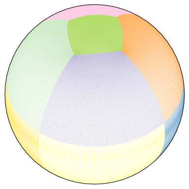
If you are not familiar with LLC grids, here is what it looks like. Different colors represent different “faces”, which aren’t necessarily parallel to each other.

Show code cell source Hide code cell source

ax = plt.axes(
    projection=ccrs.Orthographic(
        central_longitude=0.0,
        central_latitude=45.0,
    )
)
ax.scatter(lon, lat, s=0.1, c=face, transform=ccrs.PlateCarree(), cmap="Set3")
plt.show()

Every corner point is connected to 4 staggered velocity points. For MITgcm indexing, the upper and right one has the same index as the corner, so we could just read in that.

Show code cell source Hide code cell source

u = np.array(ds.UVELMASS)
v = np.array(ds.VVELMASS)

U_up = u[ind]
V_right = v[ind]

We can use the ind_tend_vec function to figure out the other two indexes for the velocity points.

The next line is going to have a warning, because some of the points we defined on continental Antarctica don’t have neighboring points. Since, they are on land, it does not matter as far as we are concerned.

ind_left = tp.ind_tend_vec(ind, 2 * np.ones_like(face), cuvwg="V")
ind_down = tp.ind_tend_vec(ind, 1 * np.ones_like(face), cuvwg="U")

Let’s just read the velocities at the other points.

U_down = u[tuple(ind_down)]
V_left = v[tuple(ind_left)]

It’s actually not as simple as that. Grids are not always parallel to each other. For example, sometimes \(U\) becomes \(V\), and \(V\) becomes \(-U\).

Well, the Topology object takes care of that as well with little additional effort.

V_down = v[tuple(ind_down)]
U_left = u[tuple(ind_left)]

fc1 = ind[0]
fc2 = ind_left[0].astype(int)
fc3 = ind_down[0].astype(int)

where = np.where(fc1 != fc3)[0]
for i in where:
    faces = np.array([fc1[i], fc3[i]])
    UfromUvel, UfromVvel, _, _ = tp.get_uv_mask_from_face(faces)
    U_down[i] = UfromVvel[1] * V_down[i] + UfromUvel[1] * U_down[i]

where = np.where(fc1 != fc2)[0]
for i in where:
    faces = np.array([fc1[i], fc2[i]])
    _, _, VfromUvel, VfromVvel = tp.get_uv_mask_from_face(faces)
    V_left[i] = VfromVvel[1] * V_left[i] + VfromUvel[1] * U_left[i]

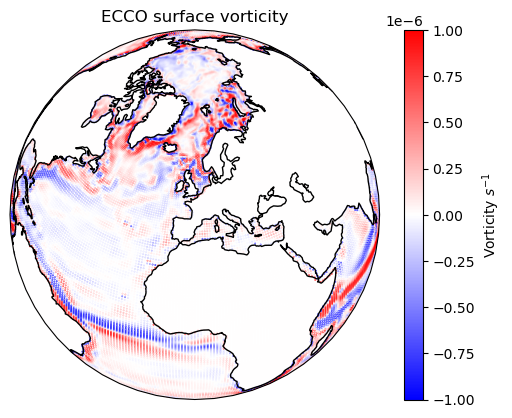
Ha, we got everything we need. Let’s calculate the velocity and plot it.

vor = (V_right - V_left) / dx + (U_down - U_up) / dy

Show code cell source Hide code cell source

ax = plt.axes(
    projection=ccrs.Orthographic(
        central_longitude=0.0,
        central_latitude=45.0,
    )
)
c = ax.scatter(
    lon,
    lat,
    s=0.1,
    c=vor,
    transform=ccrs.PlateCarree(),
    cmap="bwr",
    vmax=1e-6,
    vmin=-1e-6,
)
ax.coastlines()
ax.set_title("ECCO surface vorticity")
plt.colorbar(c, label=r"Vorticity $s^{-1}$")
plt.show()