Author: Wenrui Jiang 14 June, 2023
import matplotlib.pyplot as plt
import cartopy.crs as ccrs
from tqdm import tqdm
import numpy as np
from matplotlib.collections import LineCollection
import matplotlib as mpl
import oceanspy as ospy

import seaduck as sd

mpl.rcParams["figure.dpi"] = 600Calculate the streamlines online
First we get the dataset into OceData object with help from OceanSpy. This step requires the grid to be loaded into memory as numpy arrays and then create the cKD tree on top of that, so it’s going to take some time.
od = ospy.open_oceandataset.from_catalog("LLC4320")
ds = od._ds
oce = sd.OceData(ds)
Initiate the particles randomly, so that they’re distributed evenly on the globe. Use particles.
Source
N = int(1.5e5)
np.random.seed(4320)
xx, yy, zz = [np.random.normal(size=N) for i in range(3)]
r = np.sqrt(xx**2 + yy**2 + zz**2)
y = (np.pi / 2 - np.arccos(zz / r)) * 180 / np.pi
x = np.arctan2(yy, xx) * 180 / np.pi
x = x[y > -80]
y = y[y > -80]
z = np.ones_like(x) * (-10.0)
t = np.ones_like(x) * 10.0

ax = plt.axes(
    projection=ccrs.Orthographic(central_longitude=-20.0, central_latitude=45.0)
)
ax.plot(x, y, "o", markersize=0.1, transform=ccrs.PlateCarree())
ax.coastlines()
plt.show()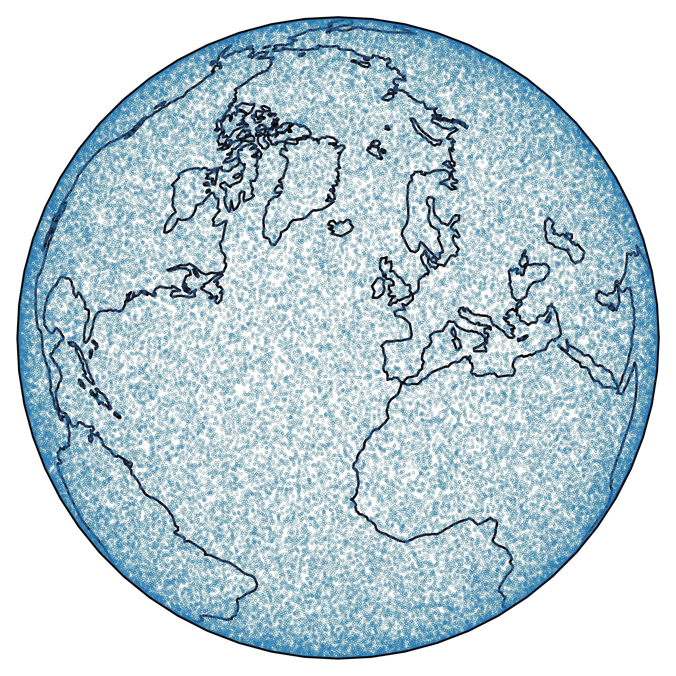
We’ll use just one vertical layer (the first one, which is at the surface) of a single snapshot (the first one) to make the streamlines.
oce["u"] = oce["U"][0, 0]
oce["v"] = oce["V"][0, 0]
By setting wname = None, we fix particles to move on a horizontal surface. Think of isobaric floats.
%%time
p = sd.Particle(
    x=x,
    y=y,
    z=z,
    t=t,
    data=oce,
    uname="u",
    vname="v",
    wname=None,
)
The package knows that LLC4320 is a large dataset, so by default it doesn’t prefetch data. Otherwise, seaduck is overwhelmed. In general, this is a smart thing to do.
However, since we are using a static 2D velocity field here, which is much smaller than the 3D time-varying field, we actually have enough memory to prefetch. So tell seaduck this bit of LLC4320 isn’t overwhelmingly big:
p.too_large = Falsep.uarray = np.array(oce["u"])
p.varray = np.array(oce["v"])Everything went well. Now, we are going to compute trajectories with a 3 hour timestep for 30 days. This will take a while: time for a nap...
step = 10800
N = 240
dest = [n * step for n in range(1, N)]
%%time
stops, raw = p.to_list_of_time(dest, update_stops=[])It took around 1.5 hours to run a month of simulation for particles. We can now extract the things we need to plot, namely longitude, latitude, and horizontal speed.
lons = np.array([i.lon for i in raw])
lats = np.array([i.lat for i in raw])
spds = np.array([np.hypot(i.u * i.dx, i.v * i.dy) for i in raw])
If you would like to save the data for plotting, you can change the following raw block to code block and run it.
np.save("LLC4320lons.npy", lons)
np.save("LLC4320lats.npy", lats)
np.save("LLC4320spds.npy", spds)
If the location and speed is already pre-computed, they can be loaded by:
lons = np.load("LLC4320lons.npy")
lats = np.load("LLC4320lats.npy")
spds = np.load("LLC4320spds.npy")
Plotting Preparation
The ETOPO topography dataset is also accessible on SciServer using OceanSpy. This will give us absolutely beautiful plots.
etopo = ospy.open_oceandataset.from_catalog("ETOPO")For this notebook, we only need the land, because there is already so much going on in the water. So clip the etopo data.
etopo = etopo._ds.where(etopo._ds.Depth > 0)Here is the function for plotting. The lines will be colored with speed. This part is going to take some time, but I hope you think it’s worth the wait.
def pretty_stream_plot(
    lats,
    lons,
    spds,
    projection,
    particle_bins=1,
    bins=5,
    north=1000,
    south=-1000,
    plot_lines=True,
    save_as=None,
):
    plt.figure(figsize=(16, 16))
    axs = plt.axes(projection=projection)
    axs.set_extent([-1e4, 1e4, south, north], crs=ccrs.PlateCarree())
    plt.tight_layout()
    axs.pcolormesh(
        etopo.X[::bins],
        etopo.Y[::bins],
        etopo.Depth[::bins, ::bins],
        transform=ccrs.PlateCarree(),
        cmap="bone",
        vmin=-3000,
        vmax=4500,
        zorder=20,
        rasterized = True,
    )
    axs.set_facecolor("lightsteelblue")
    print("finished making the map")
    if not plot_lines:
        print("skipping the lines")
        return
    # To speed up the computation, we transform the
    # latlon outside the for plotting for-loop.
    xx, yy, _ = projection.transform_points(ccrs.PlateCarree(), lons, lats).T

    xx = xx.T
    yy = yy.T

    for i in tqdm(range(0, lons.shape[1], particle_bins)):
        y = yy.T[i][1:]
        x = xx.T[i][1:]
        if np.max(x) - np.min(x) > 300:
            x[x < 0] += 360
        dydx = (0.5 * (spds.T[i][:-1] + spds.T[i][1:]))[1:]  # first derivative

        # Create a set of line segments so that we can color them individually
        # This creates the points as a N x 1 x 2 array so that we can stack points
        # together easily to get the segments. The segments array for line collection
        # needs to be (numlines) x (points per line) x 2 (for x and y)
        points = np.array([x, y]).T.reshape(-1, 1, 2)

        segments = np.concatenate([points[:-1], points[1:]], axis=1)

        # Create a continuous norm to map from data points to colors
        norm = plt.Normalize(0, 1.0)
        lc = LineCollection(segments, cmap="GnBu_r", norm=norm)
        # Set the values used for colormapping
        lc.set_array(dydx)
        lc.set_linewidth(0.3)
        lc.set_rasterized(True)
        axs.add_collection(lc)

    if save_as is not None:
plt.savefig(save_as,dpi = 300)Voila!
Looking from the Arctic
north_projection = ccrs.NorthPolarStereo(central_longitude=38.0)
pretty_stream_plot(
    lats,
    lons,
    spds,
    north_projection,
    south=6.5,
    save_as="LLC4320_files/LLC4320_29_2.png",
)
plt.show()
Fig.1 Streamlines of 150,000 particles released at 00:00 Apr 25, 2012 in LLC4320 simulated for 30 days. The color shading shows the current speed. This is looking from the North Pole.
Looking from the Antarctic
south_projection = ccrs.SouthPolarStereo(central_longitude=38.0)
pretty_stream_plot(
    lats,
    lons,
    spds,
    south_projection,
    north=-6.5,
    save_as="LLC4320_files/LLC4320_32_2.png",
)
plt.show()
Fig.2 Similar to Fig.1, but looking from the South Pole.