Vertical stream function conservation

author, Wenrui Jiang 06/06/2022

This notebook is also an idealized test for 2D flow like the horizontal case. However, it has a slightly different flavor.

This notebook looks at the vertical direction rather than the horizontal one.
We are going to simulate the particles backward in time.
The “wall” behavior of the particles are explored.

import warnings

import matplotlib as mpl
import matplotlib.pyplot as plt
import numpy as np
import xarray as xr
from matplotlib import cm, colors

import seaduck as sd

mpl.rcParams["figure.dpi"] = 300

warnings.filterwarnings("ignore")

Loading data¶

As always, we need to load the data. For simplicity and to demonstrate the capacity of particles sliding on the wall, I am going to use the stream function of an $f$ -plane gyre. You can think of this example as a zonal overturning cell in a meridional channel.

def streamfunction(x, z):
    tempz = -z / 500 - 1
    return np.cos(np.pi * x / 2) * np.cos(np.pi * tempz / 2)

N = 100
M = 50
x = np.linspace(-1, 1, N + 1)
y = np.linspace(-0.1, 0.1, 2)
zl = np.linspace(0, -1000, M)
zp1 = np.append(zl, -1001)
xg, yg = np.meshgrid(x, y)
xv = 0.5 * (xg[:, 1:] + xg[:, :-1])
yv = 0.5 * (yg[:, 1:] + yg[:, :-1])
xu = 0.5 * (xg[1:] + xg[:-1])
yu = 0.5 * (yg[1:] + yg[:-1])

xc = 0.5 * (xv[1:] + xv[:-1])
yc = 0.5 * (yv[1:] + yv[:-1])

tempx, tempz = np.meshgrid(x, zl)
strmf = streamfunction(tempx, tempz).reshape(len(zl), 1, -1)
z = 0.5 * (zp1[1:] + zp1[:-1])
zl = zp1[:-1]
drf = np.abs(np.diff(zp1))

u = np.zeros((M, 1, N + 1), float)
u[:-1] = np.diff(strmf, axis=0)
w = np.diff(strmf, axis=-1)
v = np.zeros((M, 2, N), float)

ds = xr.Dataset(
    coords=dict(
        XC=(["Y", "X"], xc),
        YC=(["Y", "X"], yc),
        XG=(["Yp1", "Xp1"], xg),
        YG=(["Yp1", "Xp1"], yg),
        Zl=(["Zl"], zl),
        Z=(["Z"], z),
        drF=(["Z"], drf),
        rA=(["Y", "X"], np.ones_like(xc, float)),
    ),
    data_vars=dict(
        UVELMASS=(["Z", "Y", "Xp1"], u),
        VVELMASS=(["Z", "Yp1", "X"], v),
        WVELMASS=(["Zl", "Y", "X"], w),
        streamfunc=(["Zl", "Yp1", "Xp1"], stream),
    ),
)
ds

Prepare the test¶

First, we convert the xarray.Dataset to seaduck.OceData

tub = sd.OceData(ds)

Now we define the initial condition of particles such that some particles are right on the wall/at the corner.

n = 30
m = 30
x = np.linspace(-1, 1, n + 1)
z = np.linspace(-0.1, -1000, m + 1)
x, z = np.meshgrid(x, z)
x = x.ravel()
z = z.ravel()

Let’s store which ones are on the wall and which ones are at the corner for plotting purposes.

on_x_wall = np.abs(x) == 1
on_z_wall = np.logical_or(z == z.min(), z == z.max())
coloring = (0.2 + np.logical_or(on_x_wall, on_z_wall)) / 1.2
corner = np.logical_and(on_x_wall, on_z_wall)

Run the test and plot¶

Finally, we can run the simulation, and plot the trajectories.

pt = sd.Particle(
    x=x, y=np.zeros_like(x), z=z, t=np.zeros_like(x), data=tub, transport=True
)

WARNING:root:Setting the surface velocity to zero. Dataset might be modified.

Again, we will look at how much the stream function changed before and after the simulation.

kkk = np.array([[0, 0], [0, 1], [1, 0], [1, 1]])

gknw = sd.KnW(kkk, vkernel="linear", tkernel="nearest")

before = pt.interpolate("streamfunc", gknw)

steps = 40
stops, ps = pt.to_list_of_time(
    normal_stops=np.linspace(0, -2 * steps * N, steps), update_stops=[]
)

1970-01-01T00:00:00
1969-12-31T23:56:35
1969-12-31T23:53:10
1969-12-31T23:49:45
1969-12-31T23:46:19
1969-12-31T23:42:54
1969-12-31T23:39:29
1969-12-31T23:36:04
1969-12-31T23:32:39
1969-12-31T23:29:14
1969-12-31T23:25:49
1969-12-31T23:22:24
1969-12-31T23:18:58
1969-12-31T23:15:33

1969-12-31T23:12:08
1969-12-31T23:08:43
1969-12-31T23:05:18
1969-12-31T23:01:53
1969-12-31T22:58:28
1969-12-31T22:55:03
1969-12-31T22:51:37
1969-12-31T22:48:12
1969-12-31T22:44:47
1969-12-31T22:41:22
1969-12-31T22:37:57
1969-12-31T22:34:32
1969-12-31T22:31:07

1969-12-31T22:27:42
1969-12-31T22:24:16
1969-12-31T22:20:51
1969-12-31T22:17:26
1969-12-31T22:14:01
1969-12-31T22:10:36
1969-12-31T22:07:11
1969-12-31T22:03:46
1969-12-31T22:00:21
1969-12-31T21:56:55
1969-12-31T21:53:30
1969-12-31T21:50:05

1969-12-31T21:46:40

after = pt.interpolate("streamfunc", gknw)

As promised, the difference is indeed very small.

is_it_close = np.allclose(after, before, atol=1e-7)
max_difference = np.max(np.abs(after - before))
print(f"Is the stream function is conserved? {is_it_close}")
print(f"The maximum difference is {max_difference }")

Is the stream function is conserved? True
The maximum difference is 1.3688851652204903e-07

for i in range(len(x)):
    if corner[i]:
        plt.plot(lons.T[i], deps.T[i], "x-", c="r")
    plt.plot(lons.T[i], deps.T[i], c=mapper.to_rgba(coloring[i]))
plt.ylabel("Depth")
plt.xlabel("X")
plt.title("Particle trajectories in a zonal overturning cell")
plt.show()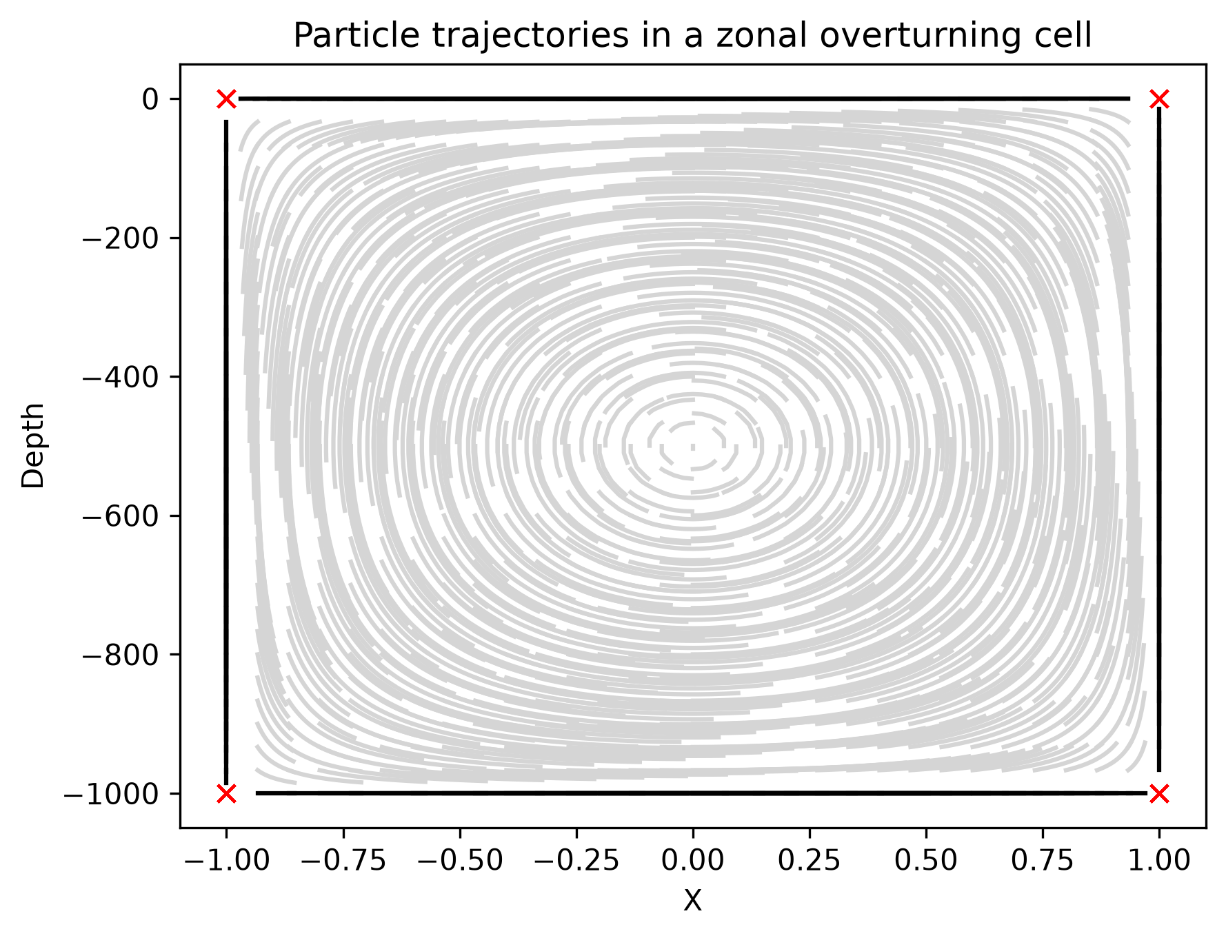

Fig.1 Particle trajectories in zonal overturning cell. Grey and black lines represent the trajectories of interior and wall attached particles, respectively. The red crosses show the trajectories of corner points.

Remarks¶

Hopefully, this has already convinced you that the paticles are conserving streamfunction in the vertical.

The non-penetrating condition means that particles on the wall will not detach in any finite time. Likewise, particles at the corners will never leave.

At the center, the point with maximum stream function has nowhere to go, so it stays there forever.