Carenza Williams & Wenrui Jiang, Feb 2026
This notebook demonstrates how to calculate the time-mean Eulerian salinity budget in ECCOv4r4, with a focus on the advection term. The method illustrated in this notebook can be found in our paper titled “Tracer Budgets on Lagrangian Trajectories”.
This is No.1 of a serie of 2 tutorial notebooks. The second one can be found here.
0.Set up
Let’s start by loading in our dataset and some key packages.
Source
# -----------------
# Import packages
# -----------------
import warnings

import numpy as np
import xarray as xr

import seaduck as sd
import seaduck.eulerian_budget as sdeb

# Suppress futurewarning
warnings.filterwarnings("ignore", category=FutureWarning,
                        message="elementwise comparison failed")
# Suppress xgcm padding warning
warnings.filterwarnings("ignore", category=UserWarning,
                        message="rename 'Z' to 'Z' does not create an index anymore")
# -----------------------------
# Load and inspect the dataset
# -----------------------------
ds_bar = sd.utils.get_dataset('eul_bud_mean')
# Create cell volume
vol = (ds_bar.rA*ds_bar.drF*ds_bar.hFacC).transpose('face','Z','Y','X')
ds_bar['Vol'] = vol
ds_barDownloading file 'eul_bud_mean.tar.gz' from 'doi:10.5281/zenodo.21536496/eul_bud_mean.tar.gz' to '/home/runner/.cache/seaduck'.
Untarring contents of '/home/runner/.cache/seaduck/eul_bud_mean.tar.gz' to '/home/runner/.cache/seaduck/eul_bud_mean.tar.gz.untar'
This dataset has the required variables to calculate the mean salinity budget, as well as some ECCOv4r4 grid variables. These are:
S_bar --> time-mean salinity [PSU]
T_bar --> time-mean potential temperature [°C]
u_bar, v_bar, w_bar --> time-mean total velocity m s []
ADVx_SLT_bar (etc.) --> time-mean advective flux of salinity [PSU m s]
DFx_SLT_bar (etc.) --> time-mean diffusive flux of salinity [PSU m s]
forcS_bar --> time-mean salt forcing [PSU s]
forcFW_bar --> time-mean freshwater forcing [PSU s]
tendSln_bar --> time-mean salinity tendency [PSU s]
spdivup_bar --> [PSU s]
The variables in the first five lines can be directly downloaded from the ECCOv4r4 website. Since this notebook focuses on the advective process, the Eulerian tendency, the eddy transport, and the forcing terms are precalculated for brevity. Interested readers are directed to Piecuch 2017 for an instructive guide on the calculation of those terms.
# Grid object
grid = sdeb.create_ecco_grid(ds_bar,for_outer = True)
1. Calculate the wall salinity
A key step to bridge the difference between Eulerian and Lagrangian frameworks is to calculate the “wall salinity”. This involves interpolating the model salinity onto the grid walls so that salinity and velocity can be stored at the same point on the model grid.
First, we will create a Topology object using a seaduck built-in function, which helps us navigate the complex tile connections of ECCO.
# Topology object
tp = sd.Topology(ds_bar)
The ECCO use third order upwind and third order direct space-time scheme for salinity advection in the vertical and horizontal, respectively. third_order_upwind_z and third_order_DST_x/y are built-in seaduck functions that mimic the behavior of those advection schemes.
# ----------------------------------------------
# Create wall salinity (uses seaduck functions)
# ----------------------------------------------

lm = 2 # The extra margin on the left side
rm = 1 # and that on the right side

dx = np.array(ds_bar.dxG)
dy = np.array(ds_bar.dyC)
ds = ds_bar

w = np.array(ds.w_bar)
s = np.array(ds.S_bar.where(ds.maskC!=0))
sz = sdeb.third_order_upwind_z(s,w)# The vertical advection scheme

u = np.array(ds.u_bar)
sx = np.zeros_like(s)
for face in range(13):
    xbuffer = sdeb.buffer_x_withface(s,face,lm,rm,tp)
    u_cfl = np.array(u[...,face,:,:]/dx[face])

    sx[:,face,:,:] = sdeb.third_order_DST_x(xbuffer,u_cfl)


v = np.array(ds_bar.v_bar)
sy = np.zeros_like(s)
for face in range(13):
    u_cfl = np.array(v[...,face,:,:]/dy[face])
    ybuffer = sdeb.buffer_y_withface(s,face,lm,rm,tp)

    sy[:,face,:,:] = sdeb.third_order_DST_y(ybuffer,u_cfl)

ds_bar['sx_bar'] = xr.DataArray(sx.reshape(50,13,90,90),dims = ('Z','face','Y','Xp1'))
ds_bar['sy_bar'] = xr.DataArray(sy.reshape(50,13,90,90),dims = ('Z','face','Yp1','X'))
ds_bar['sz_bar'] = xr.DataArray(sz.reshape(50,13,90,90),dims = ('Zl','face','Y','X'))
Now our dataset also contains the time-mean salinity stored on the x, y and z faces of the model grid. This will be required to calculate the advection term of the salinity budget.
2. Calculating the Salinity Budget
Now, onto the main event: finding the salinity budget.
The time-mean salinity budget can be expressed as:
where is calculated by:
Terms are defined as:
--> Eulerian tendency
--> (Mean) advection
--> Eddy transport
--> Diffusion of salinity
--> Freshwater forcing
--> Salt forcing (from run off, ice plume, etc.)
All terms but the advection of salinity are stored in the dataset ‘ds_bar’. We must calculate the advection of salinity term, which we will do one term at a time below.
First, we calculate volume transport from velocity.
Source
# ---------------------------
# Define transport function
# ---------------------------

def vel_to_trans(u, v, w):
    return (
        u * ds_bar.drF * ds_bar.dyG,
        v * ds_bar.drF * ds_bar.dxG,
        w * ds_bar.rA
    )
# Calculate volume transport
ut, vt, wt = vel_to_trans(ds_bar.u_bar, ds_bar.v_bar, ds_bar.w_bar)
ds_bar['utrans'] = ut.compute()
ds_bar['vtrans'] = vt.compute()
ds_bar['wtrans'] = wt.compute()
ds_bar['wtrans'][0,:] = 0We can now calculate the mean component of the salinity fluxes
ds_bar['ubarsbar_x'] = (ut * ds_bar.sx_bar).compute()
ds_bar['ubarsbar_y'] = (vt * ds_bar.sy_bar).compute()
ds_bar['ubarsbar_z'] = (wt * ds_bar.sz_bar).compute()
ds_bar['ADV_x'] = ds_bar.ADVx_SLT_bar.compute()
ds_bar['ADV_y'] = ds_bar.ADVy_SLT_bar.compute()
ds_bar['ADV_z'] = ds_bar.ADVz_SLT_bar.compute()ds_bar['DIF_x'] = (ds_bar.DFx_SLT_bar).compute()
ds_bar['DIF_y'] = (ds_bar.DFy_SLT_bar).compute()
ds_bar['DIF_z'] = (ds_bar.DFz_SLT_bar).compute()To calculate the divergence of the fluxes, we first create a OceData object
tub = sd.OceData(ds_bar)Calculate 
# -------------------------------
# Calculate div (uS)
# -------------------------------
divus = sdeb.total_div(tub, grid, 'ubarsbar_x', 'ubarsbar_y', 'ubarsbar_z')
Calculate 
# -------------------------------
# Calculate div (uS)
# -------------------------------
divu = sdeb.total_div(tub, grid, 'utrans', 'vtrans', 'wtrans')
# Multiply by mean salinity
# -------------------------------
# Calculate the term -- S div (u)
# -------------------------------
sdivu = ds_bar.S_bar * divuNow the above terms can be combined to give the required term:
Calculate 
# -------------------------------
# Calculate u dot grad(S)
# -------------------------------
ugrads = divus - sdivu
Calculate the divergence of ADV and DIF terms
# -------------------------------
# Calculate div(ADV)
# -------------------------------

divADV = sdeb.total_div(tub, grid, 'ADV_x', 'ADV_y', 'ADV_z')
# -------------------------------
# Calculate -div(DIF)
# -------------------------------
dif_h = -sdeb.hor_div(tub, grid, 'DIF_x', 'DIF_y')
dif_v = -sdeb.ver_div(tub, grid, 'DIF_z')3. Check the budget closure
# ------------------------------
# Calculate the advection term
# ------------------------------

adv = ugrads
# ------------------------------
# Calculate the eddy transport term
# ------------------------------
neg_upgradsp_bar = -(divADV - divus - ds_bar.spdivup_bar)# ------------------------------
# Calculate the total forcing term
# ------------------------------
forc = ((-ds_bar.forcFW_bar) + ds_bar.forcS_bar)Once again, we are trying to close this budget:
If we have done this correctly, then the LHS - RHS of the budget equation should equal 0 (to machine precision). Let’s check!
# ------------------------------
# Check that the budget closes
# ------------------------------

res = (ds_bar.tendSln_bar + adv) - (neg_upgradsp_bar + dif_h + dif_v + forc)
# ----------------------------------------------
# Plot the residuals (around the UK and Europe)
# ----------------------------------------------
res[0,2].plot()/home/runner/micromamba/envs/DEVELOP/lib/python3.11/site-packages/dask/_task_spec.py:768: RuntimeWarning: invalid value encountered in divide
return self.func(*new_argspec)
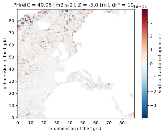
Success! The fact that the residual is very small and look random suggests that it arise solely from round-off error.
The only thing left to do now is to save our work...
Source
out = ds[['sx_bar','sy_bar','sz_bar','u_bar','v_bar','w_bar','S_bar','T_bar','dxG','dyG']]
out['neg_upgradsp_bar'] = neg_upgradsp_bar
out['forc_s'] = forc
out['dif_h'] = dif_h
out['dif_v'] = dif_v
out['conv_us'] = -divus
out['tend_s'] = ds_bar.tendSln_bar
out.to_zarr('lag_budg.zarr', mode='w', zarr_format=2)
/home/runner/micromamba/envs/DEVELOP/lib/python3.11/site-packages/dask/_task_spec.py:768: RuntimeWarning: invalid value encountered in divide
return self.func(*new_argspec)
<xarray.backends.zarr.ZarrStore at 0x7fca2c953b00>... and now we can use these eulerian budget terms to calculate the Lagrangian budget in the next notebook.
- Jiang, W., & Haine, T. W. N. (2025). Tracer Budgets on Lagrangian Trajectories. Journal of Advances in Modeling Earth Systems, 17(9). 10.1029/2024ms004848