Particles are simulated in the Southern Ocean AVISO altimetry surface-ocean velocity field.
Author: Wenrui Jiang, Tom Haine Feb '23
Source
import cartopy.crs as ccrs
import matplotlib as mpl
import matplotlib.pyplot as plt
import numpy as np

import seaduck as sd

mpl.rcParams["figure.dpi"] = 300
Loading data
The velocity field dataset is derived from AVISO sea surface height products, which were processed by SSALTO/DUACS and distributed by AVISO+ (https://seaduck.utils provides a few datasets for testing and demonstration purposes. The corresponding dataset is called when the corresponding functions are called.
ds = sd.utils.get_dataset("aviso")
ds
Downloading file 'aviso.tar.gz' from 'doi:10.5281/zenodo.15884732/aviso.tar.gz' to '/home/runner/.cache/seaduck'.
Untarring contents of '/home/runner/.cache/seaduck/aviso.tar.gz' to '/home/runner/.cache/seaduck/aviso.tar.gz.untar'
Now, create the OceData object which provides methods to translate between lat-lon and grid-oriented coords. The model coords frequently needed are also cached.
bathtub = sd.OceData(ds)The object also contains a tp (topology) object. It looks at the shape of the coordinate data. In this Southern Ocean case, based on the longitude range, it thinks the type is x_periodic, which is correct for the Southern Ocean.
bathtub.tp.typ'x_periodic'We’ve prepared the bathtub that the ducks are going to swim (passively drift) in. Now decide where and when to drop them.
We are going to use a short-hand defined in seaduck.utils to define the initial position for simplicity. The returns are normally four 1D numpy array of lon, lat, dep, and time. It’s as simple as that.
# Define the extend of the box
west = -180.0
east = 180.0
south = -74.99
north = -40.01
shallow = -10.0
deep = -10.0

time = "1970-01-01"

Nlon = 300  # How many along longitudinal direction?
Nlat = 30  # How many along latitudinal direction?
Ndep = 1  # How many along vertical direction?

x, y, z, t = sd.utils.easy_3d_cube(
    (west, east, Nlon),
    (south, north, Nlat),
    (shallow, deep, Ndep),
    time,
    print_total_number=True,
)
A total of 9000 positions are defined.
Here is where the particles start on the map:
Source
plt.figure(figsize=(16, 9))
ax = plt.axes(projection=ccrs.SouthPolarStereo(central_longitude=170.0))
ax.plot(x, y, "r+", markersize=1, transform=ccrs.PlateCarree())
ax.coastlines()
ax.set_title("Particle initial position")
plt.show()
/home/runner/micromamba/envs/DEVELOP/lib/python3.11/site-packages/cartopy/io/__init__.py:242: DownloadWarning: Downloading: https://naturalearth.s3.amazonaws.com/110m_physical/ne_110m_coastline.zip
warnings.warn(f'Downloading: {url}', DownloadWarning)
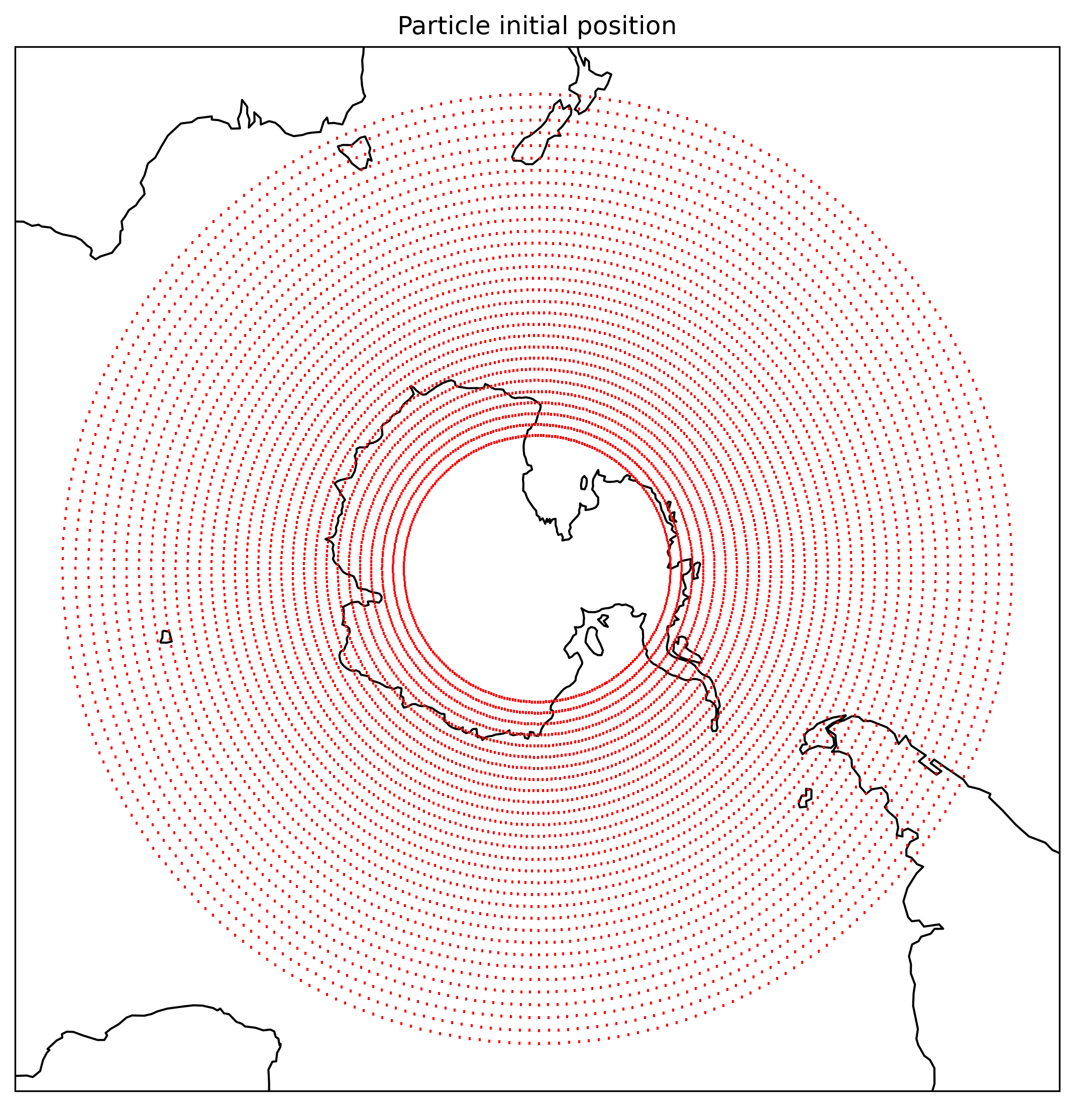
Fig.1 Initial position of the particles.
The AVISO velocity data only has the horizontal velocity component. Or in other words, all the particles are assumed to be at the same (implicit) level, which is the surface for this example. seaduck takes care of that by just setting:
z = NoneThe AVISO velocity field is a snapshot and does not have a time dimension. Therefore, the time is only valid in a relative sense, i.e. how long has the simulation gone in “real” time.
The standard format for time in seaduck is seconds since 1970-01-01 00:00, and it could be negative. Remember what time is set as the initial time?
all(t == 0)TrueLet’s now define the duration of the simulation (end before start means integrate backwards in time). We can again use a short hand from seaduck.utils.
tf = sd.utils.convert_time("1970-02-01")This is equivalent to:
tf = (np.datetime64("1970-02-01") - np.datetime64("1970-01-01")) / np.timedelta64(
    1, "s"
)
We’re not interested when particles leave the domain, so we disregard the ones that leave from the northern boundary by defining:
def interested_in(p):
    return np.logical_and(-74.5 < p.lat, p.lat < -45.5)
Create the OceInterp.lagrangian.particle object.
We have all the information we need. The final step of preparation is to create the seaduck.lagrangian.particle object. We need to tell the seaduck this information about the particles: where and when they start, which bathtub they’re in, and the names of the velocity components; because it’s not great at guessing.
p = sd.Particle(
    x=x,
    y=y,
    z=z,
    t=t,
    data=bathtub,
    uname="u",
    vname="v",
    wname=None,
    callback=interested_in,
)
p
/home/runner/work/seaduck/seaduck/seaduck/eulerian.py:991: UserWarning: No maskC in dataset. Perhaps set ds['maskC'] = ds.HFacC
warnings.warn("No maskC in dataset. Perhaps set ds['maskC'] = ds.HFacC")
<seaduck.lagrangian.Particle at 0x7fb4b5b75fd0>Perform the particle trajectory simulation.
The to_list_of_time method does the Lagrangian trajectory calculation.
Notice how we define when to dump output (normal_stops) and when to update the velocity field (update_stops). By default, the stops returned by the integration is the combination (union) of normal_stops and update_stops. raw is a list of OceInterp.eulerian.position objects with the same length as stops.
normal_stops = np.linspace(t[0], tf, 10)
stops, raw = p.to_list_of_time(normal_stops=normal_stops)
/home/runner/work/seaduck/seaduck/seaduck/utils.py:841: RuntimeWarning: invalid value encountered in divide
tl = np.log(1 - du / u * (0.5 + x0)) / du
/home/runner/work/seaduck/seaduck/seaduck/utils.py:841: RuntimeWarning: divide by zero encountered in log
tl = np.log(1 - du / u * (0.5 + x0)) / du
/home/runner/work/seaduck/seaduck/seaduck/utils.py:841: RuntimeWarning: invalid value encountered in log
tl = np.log(1 - du / u * (0.5 + x0)) / du
/home/runner/work/seaduck/seaduck/seaduck/utils.py:842: RuntimeWarning: invalid value encountered in divide
tr = np.log(1 + du / u * (0.5 - x0)) / du
/home/runner/work/seaduck/seaduck/seaduck/utils.py:842: RuntimeWarning: divide by zero encountered in log
tr = np.log(1 + du / u * (0.5 - x0)) / du
/home/runner/work/seaduck/seaduck/seaduck/utils.py:842: RuntimeWarning: invalid value encountered in log
tr = np.log(1 + du / u * (0.5 - x0)) / du
/home/runner/work/seaduck/seaduck/seaduck/utils.py:844: RuntimeWarning: divide by zero encountered in divide
tl[no_gradient] = (-x0[no_gradient] - 0.5) / u[no_gradient]
/home/runner/work/seaduck/seaduck/seaduck/utils.py:845: RuntimeWarning: divide by zero encountered in divide
tr[no_gradient] = (0.5 - x0[no_gradient]) / u[no_gradient]
/home/runner/work/seaduck/seaduck/seaduck/utils.py:790: RuntimeWarning: divide by zero encountered in divide
incr = u / du * (np.exp(du * t) - 1)
/home/runner/work/seaduck/seaduck/seaduck/utils.py:790: RuntimeWarning: invalid value encountered in divide
incr = u / du * (np.exp(du * t) - 1)
/home/runner/work/seaduck/seaduck/seaduck/utils.py:790: RuntimeWarning: invalid value encountered in multiply
incr = u / du * (np.exp(du * t) - 1)
1970-01-01T00:00:00
1970-01-04T10:40:00
1970-01-07T21:20:00
1970-01-11T08:00:00
1970-01-14T18:40:00
/home/runner/work/seaduck/seaduck/seaduck/utils.py:841: RuntimeWarning: divide by zero encountered in divide
  tl = np.log(1 - du / u * (0.5 + x0)) / du
/home/runner/work/seaduck/seaduck/seaduck/utils.py:842: RuntimeWarning: divide by zero encountered in divide
  tr = np.log(1 + du / u * (0.5 - x0)) / du
1970-01-18T05:20:00
1970-01-21T16:00:00
1970-01-25T02:40:00
1970-01-28T13:20:00
1970-02-01T00:00:00
Plotting
First we extract the longitude and latitude from the raw object.
lons = np.array([pt.lon for pt in raw]).T
lats = np.array([pt.lat for pt in raw]).T
Some particles passed through the dateline (periodic boundary). Here is some post-processing to handle the plot.
Source
for i in range(len(lons)):
    diff = np.diff(lons[i])

    if max(abs(diff)) > 330:
        for j in np.where(abs(diff) > 300)[0]:
            j = int(j)
            lons[i, j + 1 :] -= np.sign(diff[j]) * 360
Voila!
Source
plt.figure(figsize=(9, 16))
ax = plt.axes(projection=ccrs.SouthPolarStereo(central_longitude=170.0))
ax.plot(lons.T, lats.T, "darkblue", lw=0.3, transform=ccrs.PlateCarree())
ax.coastlines()
ax.set_title("Particle trajectories")
plt.show()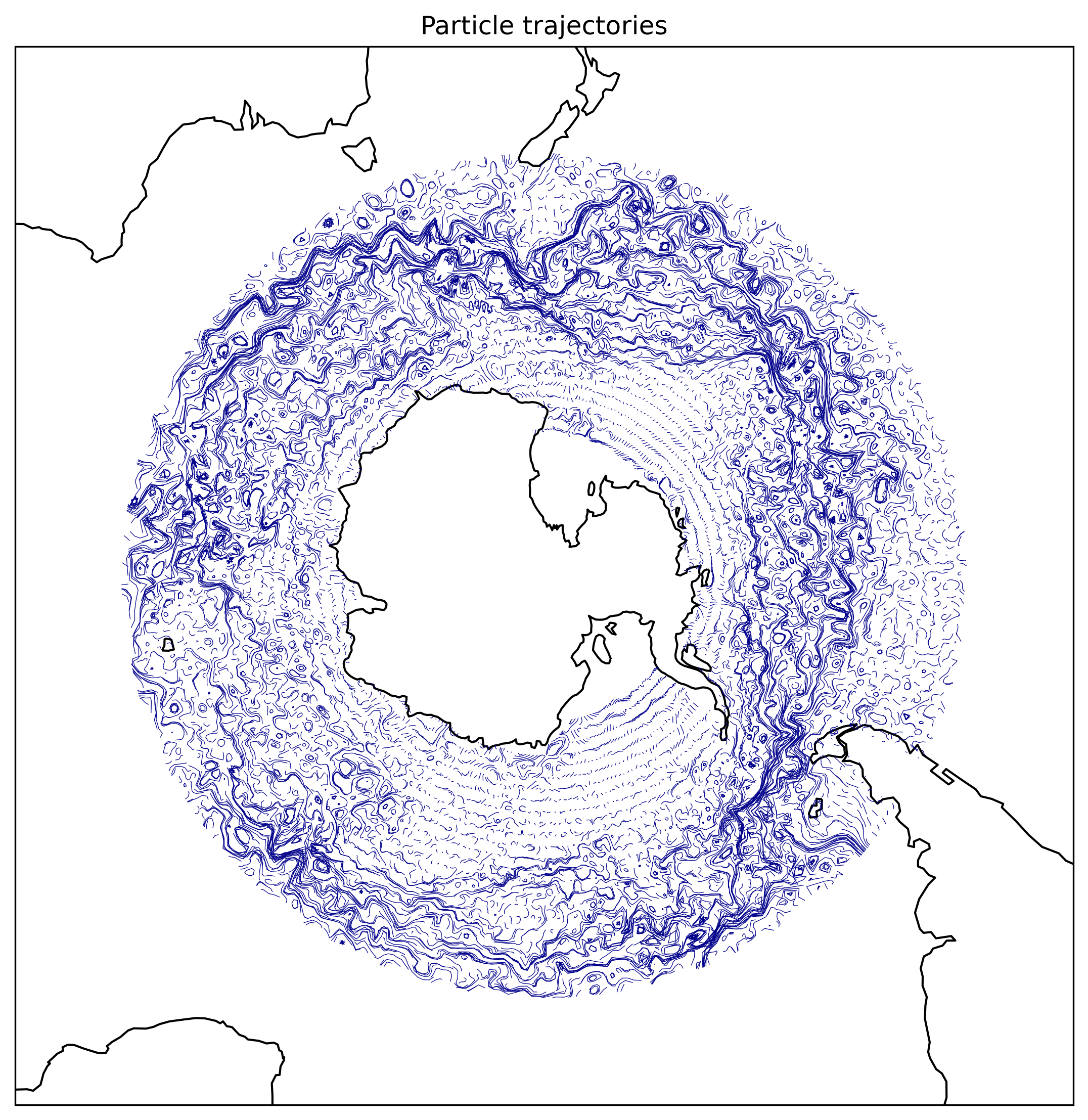
Fig.2 The trajectories of particles advected by AVISO-derived surface velocity field.
Advanced use of Particle
In this subsection, we are going to demonstrate how to access the analytical trajectories of particles. We are also going to demonstrate the flexibility of Particle release.
Most of the notebooks release particles at the same time. We are going to do it differently this time. They are going to be released at 64W and 55S and 64S. Crucially, all of the particles are released at a different time.
Source
N = 777
t_earliest = sd.utils.convert_time("1970-01-01")
t_final = sd.utils.convert_time("1970-02-01")
t_latest = sd.utils.convert_time("1970-03-03")  # damn you, February.
t = np.linspace(t_earliest, t_latest, N)

number_of_loop = 6.18
# y = -65.0+np.abs(10-np.linspace(0,number_of_loop*20,N)%20)
y = -59.5 + 4.5 * np.sin(number_of_loop * np.linspace(-3.14, 3.14, N))
x = np.ones(N) * (-64.0)
z = -np.ones(N)
To better demonstrate, here is a plot showing the release pattern of the particle. The time is referenced against the final time of the simulation. Note that every single particle will be released at a different time and there are going to be both forward and backward particles in the same simulation.
This is as if there is a ship is commuting in drake passage while releasing particles.
Source
plt.plot(t, y, "o", markersize=1)
plt.xticks(
    [t_earliest, t_final - 15 * 86400, t_final, t_final + 15 * 86400, t_latest],
    ["-31 days", "-15 days", "0", "+15 days", "+31 days"],
)
plt.ylabel("Latitude")
plt.title("Latitude of particles released at 64W")
plt.show()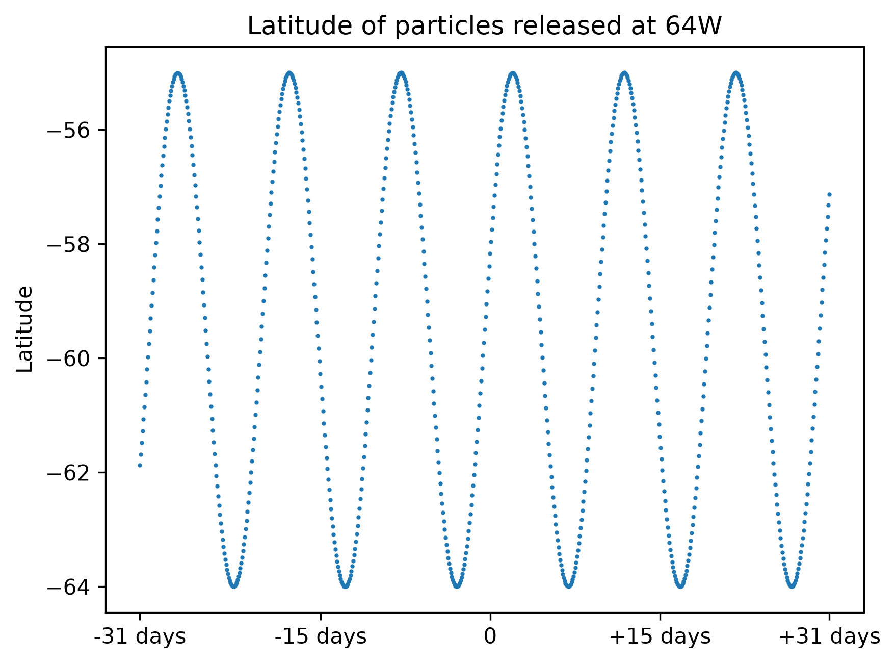
Fig.3 Pattern of particle release. Time is relative to the final time.
The only difference in preparation between this one and the previous simulation is that we have save_raw = True. This means the particles will record all the necessary informations to reconstruct the analytical trajectory.
p = sd.Particle(
    x=x,
    y=y,
    z=z,
    t=t,
    data=bathtub,
    uname="u",
    vname="v",
    wname=None,
    callback=interested_in,
    save_raw=True,
)
/home/runner/work/seaduck/seaduck/seaduck/eulerian.py:991: UserWarning: No maskC in dataset. Perhaps set ds['maskC'] = ds.HFacC
warnings.warn("No maskC in dataset. Perhaps set ds['maskC'] = ds.HFacC")
No tricks need to be played while execution.
%%time
p.to_next_stop(t_final)
/home/runner/work/seaduck/seaduck/seaduck/utils.py:841: RuntimeWarning: invalid value encountered in log
tl = np.log(1 - du / u * (0.5 + x0)) / du
/home/runner/work/seaduck/seaduck/seaduck/utils.py:841: RuntimeWarning: invalid value encountered in divide
tl = np.log(1 - du / u * (0.5 + x0)) / du
/home/runner/work/seaduck/seaduck/seaduck/utils.py:842: RuntimeWarning: invalid value encountered in divide
tr = np.log(1 + du / u * (0.5 - x0)) / du
/home/runner/work/seaduck/seaduck/seaduck/utils.py:842: RuntimeWarning: invalid value encountered in log
tr = np.log(1 + du / u * (0.5 - x0)) / du
/home/runner/work/seaduck/seaduck/seaduck/utils.py:844: RuntimeWarning: divide by zero encountered in divide
tl[no_gradient] = (-x0[no_gradient] - 0.5) / u[no_gradient]
/home/runner/work/seaduck/seaduck/seaduck/utils.py:845: RuntimeWarning: divide by zero encountered in divide
tr[no_gradient] = (0.5 - x0[no_gradient]) / u[no_gradient]
/home/runner/work/seaduck/seaduck/seaduck/utils.py:790: RuntimeWarning: divide by zero encountered in divide
incr = u / du * (np.exp(du * t) - 1)
/home/runner/work/seaduck/seaduck/seaduck/utils.py:790: RuntimeWarning: invalid value encountered in multiply
incr = u / du * (np.exp(du * t) - 1)
/home/runner/work/seaduck/seaduck/seaduck/utils.py:790: RuntimeWarning: invalid value encountered in divide
incr = u / du * (np.exp(du * t) - 1)
/home/runner/work/seaduck/seaduck/seaduck/utils.py:842: RuntimeWarning: divide by zero encountered in log
tr = np.log(1 + du / u * (0.5 - x0)) / du
CPU times: user 1.31 s, sys: 23 ms, total: 1.33 s
Wall time: 1.33 s
/home/runner/work/seaduck/seaduck/seaduck/lagrangian.py:794: UserWarning: maximum iteration count reached
  warnings.warn("maximum iteration count reached")
When save_raw = True is selected, the Particle object records location and velocity information everytime velocity is updated. The following plot is plotted from longitude and latitudes of particles crossing cell walls. Each trajectory is colored based on the time of release, Purple is the earliest, red is the latest (furthest into the future).
Source
plt.figure(figsize=(9, 16))
ax = plt.axes(projection=ccrs.PlateCarree())
rainbow = plt.get_cmap("rainbow")
for i in range(0, N):
    color = rainbow(t[i] / 2 / t_final)
    ax.plot([x[i]] + p.xxlist[i], [y[i]] + p.yylist[i], color=color, lw=0.2)
ax.coastlines()
plt.show()
/home/runner/micromamba/envs/DEVELOP/lib/python3.11/site-packages/cartopy/io/__init__.py:242: DownloadWarning: Downloading: https://naturalearth.s3.amazonaws.com/10m_physical/ne_10m_coastline.zip
warnings.warn(f'Downloading: {url}', DownloadWarning)
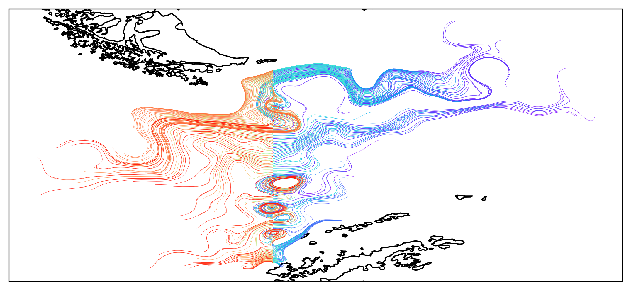
Fig.4 Trajectory of particles released at different time. Warm color are particles released after the final time, and cold colors are those released before the final time.